DEF CON 33 - Quantum Village - The Shapiro Incident

Introduction

Quantum Key Distribution (QKD) is often described as “unhackable” because, in the ideal model, any eavesdropper who touches the qubits disturbs them and gets caught. The Shapiro Incident challenge from DEF CON’s Quantum Village is another reminder that real systems live in the non-ideal world. Similar to The Entropy Heist challenge which introduced operational implementation failures of Post-Quantum Cryptography, Professor Shapiro didn’t break the quantum mechanics of the system. She listened to something the math doesn’t talk about: the analog whisper, or operational side-channel, of Bob’s detector.

This post is an end-to-end dive into how that whisper becomes a leak. We’ll start with the data we were given, walk through how a single physical parameter, avalanche charge amplitude, quietly biases the surviving bits, and show how a simple alignment step turns a biased subsequence into readable ASCII. Along the way we’ll detour through avalanche photodiode physics, sifting, timing/jitter, byte-phase alignment, and why 70% wasn’t a magic number but the right trade-off for this dataset. The conclusion is a flag and, more importantly, a lesson: math proves what could be secure, but implementation decides what is actually secure.

Initial Data

Let’s take a look at the initial data we were given for the challenge.

The challenge provided four files. The one that looks most important at first glance is the session exchange log, representing the full QKD data exchanged:

$ head exchange_obf.csv 
pid,bA,vA,bB,vB
0,X,1,Z,1
1,X,1,Z,0
2,Z,1,X,0
3,X,1,Z,1
4,Z,1,Z,1
5,X,1,Z,1
6,Z,1,X,1
7,Z,0,Z,0
8,Z,0,X,1

We’re also provided with additional files representing equipment measurements. This is classical telemetry data surrounding the QKD process:

The detector_temp.csv file logs temperature at incremental time steps.

$ head detector_temp.csv 
time_s,temp_C
0.0,19.994035731013444
0.1,20.013472168559606
0.2,20.00529588519303
0.3,20.018023330734938
0.4,20.00415280982704
0.5,20.00977831400866
0.6,19.990905067747388
0.7,20.01350459379726
0.8,20.000599307627574

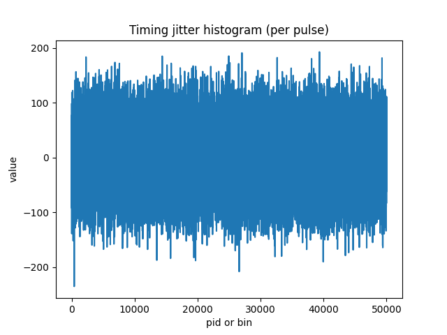
The timing_jitter.npy file summarizes the distribution of detection times per pulse.

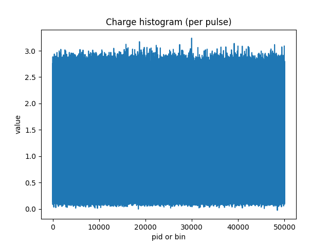
The charge_histogram.npy file is one real number per pulse: the integrated charge from Bob’s avalanche photodiodes (APDs) readout.

We have a trove of data, excellent. Let’s refresh how QKD works before diving into the specifics of the Shapiro Incident.

Background on QKD

I go more into detail of QKD theory in one of my previous posts Quantum Challenge 2020, but to summarize here:

• Alice choses a value and prepares qubits in one of two possible bases (Z or X), then sends them off to Bob.
• Bob measures the qubits in either randomly chosen basis.
• They publicly reveal their chosen bases and keep only the matching ones.
• Error rates are checked, privacy amplification happens, and a shared key emerges.

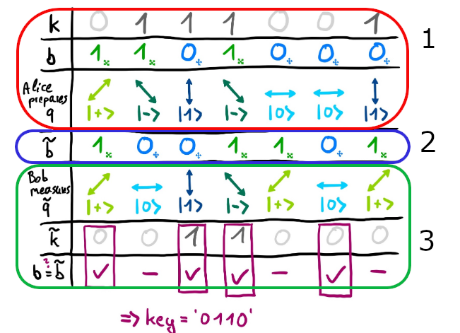
Critically, Bob’s measurement outcome is supposed to be random from Eve’s perspective. Without disturbing the quantum channel, which would raise the Quantum Bit Error Rate (QBER), there should be no way to know his raw bit string.

But this “perfect” view assumes ideal detectors. We have been given classical instrumentation telemetry that reveals imperfections in the detection process.

Glitch In The Matrix

This was one of the cooler aspects of this challenge for me. While I was already familiar with QKD and the BB84 protocol, I hadn’t spent much time digging into real-world implementations. This challenge allowed me to learn more about the operational, noisy, side of things.

When you start looking up how QKD is built in practice, you see there are a few main “categories”. Many modern high-end implementations use superconducting nanowire single-photon detectors (SNSPDs). These are efficient and low-noise, but they require cryogenic cooling and very careful infrastructure. By contrast, deployed and field-trialed fiber-based QKD systems in the 2000s–2010s use InGaAs/InP avalanche photodiodes (APDs), because they work at telecom wavelengths and can be operated with fast gating electronics at room temperature.

The avalanche multiplication process is inherently messy. The exact gain depends on microscopic noise, bias voltage, and gate timing, and this opens cracks an attacker can exploit. For example, the blinding attacks show that if you shine strong continuous light on an APD, you can force it out of single-photon mode and into a classical linear regime. Suddenly the “quantum” detector is just a photodiode under your control. Time-shift attacks exploit the fact that detector efficiencies aren’t perfectly symmetric, if you send photons slightly earlier or later, you bias which detector is more likely to fire, leaking key information. Afterpulse exploitation leverages the fact that an avalanche leaves behind trapped carriers in the diode that can re-trigger spurious clicks a few nanoseconds later, which an attacker can statistically manipulate. And ultimately in this challenge, we saw charge-amplitude biasing, where the analog height of the avalanche pulse leaks information about which detector (and thus which bit) was detected.

The tell is the charge_histogram.npy. Only APDs produce indiscriminate charge amplitudes which tend to have slightly mismatched tails depending on which detector channel clicked (corresponding to “bit=0” vs “bit=1”). We will see in the next section how we can take advantage of this to extract data.

To help illustrate what we are working with here is an example schematic of an implementation of a QKD system showing the different APDs. Red circle emphasis added.

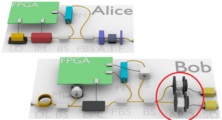
Schematic diagram of main components of the QKD system, showing the transmitter (Alice) and receiver (Bob). LD: Laser diode, IM: Intensity modulator, BS: Beam splitter, PBS: Polarising beam splitter, A: Variable optical attenuator, I: Optical isolator, F: Narrow band pass optical filter, DL: Delay line, MD: Monitoring detector, EPC: Electronic polarisation controller, FS: Fibre stretcher, APD: Avalanche photodiode detector, SD: self-differencing circuit. [1].

Why A Louder Click Gives Away A Little More

Real detectors are not twins. While the two bit channels sit behind identical APDs, environmental factors mean one channel will have a slightly larger high-amplitude tail or a slightly different gain.

If you look at the distribution of charge amplitudes when Bob reports vB=0 versus vB=1, the histograms overlap almost completely, but not perfectly. The difference is nearly invisible by eye in the bulk of the distribution but it becomes measurable in the tail where avalanches are loudest.

Let’s look at the charge_histogram.npy file a bit closer. I split the sifted clicks (throwing away where the basis didn’t match or output was -1) by Bob’s bit and plotted their charge distributions with three vertical cutoffs: 50%, 70%, and 90%.

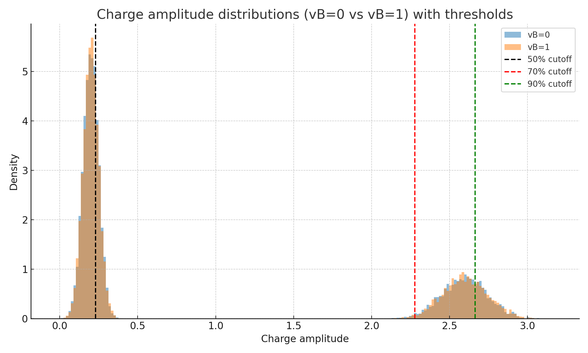
If you stare at those curves long enough you still won’t see a gap, trust me I tried…hard. But that’s the point, the difference is minor to the point of not being immediately obvious. Here is the breakdown for a series of cutoffs and the resulting bit distributions:

Percentile cutoff	Threshold	# Bits kept	Fraction 0	Fraction 1
50 (median)	0.229	12,552	0.500	0.500
70	2.278	7,531	0.497	0.503
80	2.540	5,021	0.496	0.504
90	2.665	2,511	0.492	0.508
95	2.741	1,256	0.474	0.526

Now the leakage starts to show up. At 50% the sequence is basically a fair coin: ~50/50. As you raise the cutoff and keep only louder avalanches the distribution skews, topping 52.6% ones vs 47.4% zeros at the highest cutoffs.

If you take all bits, you see random garbage. The higher the cutoff, the more pronounced the bias, however the less data to work with. We need to find the middle ground. If you select only the tail, which based on our graph above is around 70%, we’re left with a slightly unfair coin, but enough data to work with. When you concatenate tens of thousands of those bits, the bias is enough to “shine through”, as we will see when we align the stream into bytes as part of the challenge.

I Reject Your Reality, And Substitute My Own

Alright, let’s get to solving this. I’ll provide the script locations at the end of the post, but to start, we need to do a few things:

• Load the files programatically
• Sift the bits by vB != -1 and bA == bB
• Select the charge tail of the distribution based on the chosen cutoff
• Pack the bits into bytes
• Profit?

With the first attempt coded up, I gave it a shot. And…

python qv_extract_flag.py --exchange exchange_obf.csv --charge charge_histogram.npy --pct 70
[info] total pulses: 50000
[info] kept after sifting (vB>=0 & bA==bB, basis=ALL): 25103
[info] |charge| percentile 70.0 -> threshold = 2.27778
[info] selected pulses: 7531 (30.0% of sifted-in-basis)
[miss] No fully-printable qv{...} found
[peek] preview: qv{p................R........l........I....8..q.h....A%Y.T&R.......v.&..oh..k......2.4.......m...:....o........q.5.>...x.c#.K...

…oof, so close! It’s starting with qv{p so we’re clearly on to something here. What went wrong?

The reason is subtle. By filtering on charge, we’re no longer taking a perfectly contiguous run of the raw sifted key. Instead, we’re cherry-picking pulses with stronger analog signatures. That makes the distribution biased (good for us) but it also means we’re occasionally dropping or inserting a bit relative to the true byte framing. Even a single skipped bit causes every subsequent byte boundary to shift.

So what do we do? Resynchronization!

To realign the bits, we need to find the initial byte boundary and then adjust for any slips that occurred during the filtering process. Instead of assuming the byte framing will hold forever, we allow the decoder to slip by one bit whenever the output stops looking plausible.

When decoding produces non-printable garbage, shift the phase forward by one bit and keep going. This effectively re-locks onto the true framing, just like nudging those typewriter gears back into place. With this adjustment, the script can tolerate occasional skips or drops caused by the charge-threshold selection.

Alright, let’s give it another shot!

python qv_extract_flag_resync.py --exchange exchange_obf.csv --charge charge_histogram.npy --pct 70  
[info] total pulses: 50000
[info] kept after sifting (vB>=0 & bA==bB, basis=ALL): 25103
[info] |charge| percentile 70.0 -> threshold=2.27778
[info] selected pulses: 7531 (30.0% of sifted-in-basis)
[hit] initial 'qv{' at phase=0, byte_pos=0, bit_pos=0
[FLAG] qv{photon_numbar_splitters_ne6er_die}
[resync] slips_used=1
[done]

Heck yeah! So in theory our flag is qv{photon_numbar_splitters_ne6er_die}. I submit it…and still not correct. Drat. But that’s close enough that I made a small assumption that a few of the characters needed to be swapped.

I figured I would need to take out the leetspeak, bringing us to qv{photon_number_splitters_never_die}. Mic drop it was accepted, for a successful flag, and first blood on the track!

I also find the flag funny as photon number splitting (PNS) is another real attack vector against QKD. Subtle nod, it was excellent.

Summary

I loved this challenge because it rewards curiosity about how things actually work. In BB84 theory, Eve cannot gain information without disturbing the quantum states and raising the error rate - ultimately causing detection. But what we were exploiting here did not interfere with the quantum nature of QKD. It was the noisy, analog, classical layer where photons become voltages and voltages become bits.

That distinction is critical. Quantum cryptography’s promise lies in its foundations, but the real-world deployments live or die by the engineering: imperfect detectors, electronics with bias, thresholds set by humans. Side-channel attacks like this QKD hack is a reminder that most of the time it’s not the math that fails, it’s the implementation.

I want to thank Quantum Village, and specifically Robin Descamps for putting this challenge together. These kinds of challenges are rare and invaluable because they force us not just to read about QKD in papers, but to play with its guts, to grapple with how APDs or basis sifting or charge amplitudes really behave. That process deepens understanding in a way that no lecture or textbook can.

Thanks folks, until next time!

The full scripts to what I covered above can be found at https://github.com/padraignix/quantum-challenges.