
Introduction
Quantum Computing has long interested me - I mention the topic glancingly in my about page when I mentioned "where we are headed" in reference to the future of cryptographic systems. Since those teenage years I have refined that interest in an attempt to understand the underlying mechanics, the theoretical applications, and now their practical implementations. I am by no stretch of the imagination an expert on the topic and I appologize ahead of time for any glaring errors or omissions.
There is no easy way to play with quantum computing - or at least that is what I thought. I was recently introduced to qiskit, a framework that allows individuals to program and interact with quantum circuits through simulation and this completely opened my mind to further posibilities. This article is my attempt to demystify basic quantum computing concepts and allow individuals an opportunity to step through a simplistic practical implementation using qiskit with enough knowledge to be able to continue exploring themselves.
Quantum Concepts
Before we start talking about quantum gates and how to code quantum circuits practically, we need to start with some basic concepts.
Qubit
The qubit is the basic unit quantum information - the quantum equivalent of the binary digit we are used to in computer science. A qubit represents a two-state quantum mechanical system and it can be represented by the spin of a single electron such as spin up or spin down - or the quantum state. This is represented mathematically by orthonormal basis states, usually denoted as:
$$ \begin{align*} \left| 0 \right> = \left[ \begin{array}{c} 1 \\ 0 \end{array} \right] & \space \space \space \left| 1 \right> = \left[ \begin{array}{c} 0 \\ 1 \end{array} \right] \end{align*} $$
"Bra-ket" notation is used as common notation within quantum mechanics. \(\left| 0 \right>\) and \(\left| 1 \right>\) can be references as "ket 0" and "ket 1" and denote a vector in an abstract space.
Superposition
While a classical binary bit is always exactly either a 0 or 1 a qubit can simultaneously be both \(\left| 0 \right>\) or \(\left| 1 \right>\) - otherwise called a superposition of both states. A qubit can be in one of two states and the general state is a combination, or coherent superposition, of these possibilities. A pure qubit state can therefore be represented as:
$$ \begin{align*} \left| \psi \right> = \alpha\left| 0 \right> + \beta \left| 1 \right> \end{align*} $$
Where \(\alpha\) and \(\beta\) represent complex number coefficients that describe how much goes into each ket.
Entanglement
Another difference between classical bits and quantum qubits is the ability for qubits to become entangled. Entanglement can be considered a strong correlation between quantum particles to the point that they are perfectly linked even at large distances. This happens when a group of particles can only be described by the quantum state of the system rather than the individual quantum state of the particles.
To expand on the concept let's use the example of a two qubit Bell state. Mathematically this would be represented as:
$$ \begin{align*} \left|\phi^+\right> = \frac{1}{\sqrt{2}}(\left|00\right> + \left|11\right>) \end{align*} $$
Where there is an equal probability that the overall state is measured as \(\left|00\right>\) or \(\left|11\right>\). We don't know the what the first qubit would be, however we do know that they are linked. If the qubits are separated and the first is measured as a \(\left|0\right>\), then the second qubit will also be \(\left|0\right>\). We will go through a practical example of how this works later on when we work with qiskit.
Now that we have a basic understanding of the fundamentals, let us move on to how to leverage these concepts through quantum logical gates.
Quantum Gates
Before we finally get to the practical coding we will suffer through a little bit more math. Rather than just take the assumption that a logic gate performs a specific action as is, I wanted to take the opportunity and go through the "how" it actually works. This is not necessarily required to leverage the gate in a practical coding situation, yet I believe going through the math behind the action helps contextualize the code more clearly in future sections.
Similar to how classic logic gates form larger digital circuits, quantum logic gates operate on a small number of qubits and can be joined together to form quantum circuits.
Pauli X Gate
Starting off with a quantum gate that translates conceptually well to a classical equivalent - the Pauli X gate. Acting on a single qubit the Pauli X gate is the quantum equivalent of the classic NOT gate. Mathematically it is represented as:
$$ \begin{align*} \mathbb X = \begin{bmatrix} 0 & 1 \\ 1 & 0 \end{bmatrix} \end{align*} $$
We can step through two iterations to show exactly how it operates on qubits.
$$ \begin{align*} \mathbb X\left|0\right> = \begin{bmatrix} 0 & 1 \\ 1 & 0 \end{bmatrix} \left|0\right> = \begin{bmatrix} 0 & 1 \\ 1 & 0 \end{bmatrix} \begin{bmatrix} 1 \\ 0 \end{bmatrix} = \begin{bmatrix} 0 \\ 1 \end{bmatrix} = \left|1\right> \end{align*} $$
And if we start with a ket 1:
$$ \begin{align*} \mathbb X\left|1\right> = \begin{bmatrix} 0 & 1 \\ 1 & 0 \end{bmatrix} \left|1\right> = \begin{bmatrix} 0 & 1 \\ 1 & 0 \end{bmatrix} \begin{bmatrix} 0 \\ 1 \end{bmatrix} = \begin{bmatrix} 1 \\ 0 \end{bmatrix} = \left|0\right> \end{align*} $$
As we can see, applying a Pauli X gate to a qubit "bit flips" it with respect to the standard basis \(\left|0\right>\) and \(\left|1\right>\).
Hadamard Gate
The Hadamard gate brings to life the concept of superposition. The premise is simple - no matter whether we start with a ket 0 or a ket 1, by going through the Hadamard gate, the output will be in a superposition state. Let's start with defining the gate in its mathematical equivalent:
$$ \begin{align*} \mathbb H = \frac{1}{\sqrt{2}} \begin{bmatrix} 1 & 1 \\ 1 & -1 \end{bmatrix} \end{align*} $$
Now how does this make either a \(\left|0\right>\) or \(\left|1\right>\) become a superposition? Let us step through both examples and see. First what happens when the Hadamard gate is applied on \(\left|0\right>\):
$$ \begin{align*} \mathbb H\left|0\right>\ = \frac{1}{\sqrt{2}} \begin{bmatrix} 1 & 1 \\ 1 & -1 \end{bmatrix} \left|0\right> = \frac{1}{\sqrt{2}} \begin{bmatrix} 1 & 1 \\ 1 & -1 \end{bmatrix} \begin{bmatrix} 1 \\ 0 \end{bmatrix} \end{align*} $$
Which ultimately comes out to:
$$ \begin{align*} \frac{1}{\sqrt{2}} \begin{bmatrix} 1 \\ 1 \end{bmatrix} = \begin{bmatrix} \frac{1}{\sqrt{2}} \\ \frac{1}{\sqrt{2}} \end{bmatrix} \end{align*} $$
What this means is that the qubit now has a \(\begin{pmatrix}\frac{1}{\sqrt{2}}\end{pmatrix}^2 = \frac{1}{2}\) chance of being \(\left| 0 \right>\) and a \(\begin{pmatrix}\frac{1}{\sqrt{2}}\end{pmatrix}^2 = \frac{1}{2}\) chance of being \(\left| 1 \right>\). Essentially, it has an equal chance of being either and is considered in a state of superposition.
Now, if we similarly apply a Hadamard gate on \(\left|1\right>\):
$$ \begin{align*} \mathbb H\left|1\right>\ = \frac{1}{\sqrt{2}} \begin{bmatrix} 1 & 1 \\ 1 & -1 \end{bmatrix} \left|1\right> = \frac{1}{\sqrt{2}} \begin{bmatrix} 1 & 1 \\ 1 & -1 \end{bmatrix} \begin{bmatrix} 0 \\ 1 \end{bmatrix} \end{align*} $$
Then this comes out to:
$$ \begin{align*} \frac{1}{\sqrt{2}} \begin{bmatrix} 1 \\ -1 \end{bmatrix} = \begin{bmatrix} \frac{1}{\sqrt{2}} \\ \frac{-1}{\sqrt{2}} \end{bmatrix} \end{align*} $$
Similar to before, this means that the qubit has a \(\begin{pmatrix}\frac{1}{\sqrt{2}}\end{pmatrix}^2 = \frac{1}{2}\) chance of being \(\left| 0 \right>\) and a \(\begin{pmatrix}\frac{-1}{\sqrt{2}}\end{pmatrix}^2 = \frac{1}{2}\) chance of being \(\left| 1 \right>\). A state of superposition.
CNOT Gate
Alright, let's knock it up a knotch! So far we have looked at two gates that operate on a single qubit. The CNOT gate works on 2 or more qubits (we will keep it to two for this example) and additionally implements the concept of entanglement.
Assuming two qubits that are passed through \(\mathbb H\) gates we can reasonably assume that both qubits can be either \(\left|0\right>\) or \(\left|1\right>\) and there is no entanglement between the qubits. Therefore the overall state can equally represented by the basis \(\left|00\right>\),\(\left|01\right>\),\(\left|10\right>\),\(\left|11\right>\).
A CNOT gate works by using the first qubit as a control and the second qubit as the target. When the first qubit is evaluated as \(\left|1\right>\) the gate performs a NOT on the second qubit. Otherwise when the first control qubit is \(\left|0\right>\) the target qubit is left unchanged. Mathematically the CNOT gate can be defined as follows using the same above basis:
$$ \begin{align*} \mathbb Cnot = \begin{bmatrix} 1 & 0 & 0 & 0 \\ 0 & 1 & 0 & 0 \\ 0 & 0 & 0 & 1 \\ 0 & 0 & 1 & 0 \end{bmatrix} \end{align*} $$
Now let us step through the examples.
$$ \begin{align*} \mathbb Cnot\left|00\right> = \begin{bmatrix} 1 & 0 & 0 & 0 \\ 0 & 1 & 0 & 0 \\ 0 & 0 & 0 & 1 \\ 0 & 0 & 1 & 0 \end{bmatrix} \begin{bmatrix} 1 \\ 0 \\ 0 \\ 0 \end{bmatrix} = \begin{bmatrix} 1 \\ 0 \\ 0 \\ 0 \end{bmatrix} = \left|00\right> \end{align*} $$ $$ \begin{align*} \mathbb Cnot\left|01\right> = \begin{bmatrix} 1 & 0 & 0 & 0 \\ 0 & 1 & 0 & 0 \\ 0 & 0 & 0 & 1 \\ 0 & 0 & 1 & 0 \end{bmatrix} \begin{bmatrix} 0 \\ 1 \\ 0 \\ 0 \end{bmatrix} = \begin{bmatrix} 0 \\ 1 \\ 0 \\ 0 \end{bmatrix} = \left|01\right> \end{align*} $$
So far so good. When the first qubit is \(\left|0\right>\) the second qubit is not touched. Now let us perform the remaining two iterations when the first qubit is \(\left|1\right>\).
$$ \begin{align*} \mathbb Cnot\left|10\right> = \begin{bmatrix} 1 & 0 & 0 & 0 \\ 0 & 1 & 0 & 0 \\ 0 & 0 & 0 & 1 \\ 0 & 0 & 1 & 0 \end{bmatrix} \begin{bmatrix} 0 \\ 0 \\ 1 \\ 0 \end{bmatrix} = \begin{bmatrix} 0 \\ 0 \\ 0 \\ 1 \end{bmatrix} = \left|11\right> \end{align*} $$ $$ \begin{align*} \mathbb Cnot\left|11\right> = \begin{bmatrix} 1 & 0 & 0 & 0 \\ 0 & 1 & 0 & 0 \\ 0 & 0 & 0 & 1 \\ 0 & 0 & 1 & 0 \end{bmatrix} \begin{bmatrix} 0 \\ 0 \\ 0 \\ 1 \end{bmatrix} = \begin{bmatrix} 0 \\ 0 \\ 1 \\ 0 \end{bmatrix} = \left|10\right> \end{align*} $$
As we can see the second qubit is indeed flipped.
Alright no more pure math, I promise! With the understanding we have come to above we can now move on to the practical implementation and using qiskit to run our very own quantum circuits.
Qiskit Framework
Qiskit defines itself as "an open-source quantum computing software development framework for leveraging today's quantum processors". It is a a python framework that allows us to develop, graph, and simulate quantum computing circuits locally while also providing a way to integrate with IBMQ - running our developed circuits on physical quantum computers distributed around the world.
This was a game changer for me. I have been reading Quantum Computing papers on and off for awhile now, however this was purely conceptual and when trying to understand how it would work in a practical sense I would fall a bit short. Qiskit allowed me to take those concepts and do exactly that - apply them in a practical scenario, albeit it a simulated environment locally.
Environment Setup
Getting the framework setup was probably the simplest part of this entire exercise. Qiskit itself has a get started page and it essentially boils down to two module installs.
pip install qiskit
pip install qiskit-terra[visualization]
Once complete you can run a quick command to validate the install is valid and to show the various component versions. At the time of writing these are the most recent versions available.
Python 3.7.2 (tags/v3.7.2:9a3ffc0492, Dec 23 2018, 23:09:28) [MSC v.1916 64 bit (AMD64)] on win32
Type "help", "copyright", "credits" or "license" for more information.
>>> import qiskit
>>> qiskit.__qiskit_version__
{'qiskit-terra': '0.12.0',
'qiskit-aer': '0.4.0',
'qiskit-ignis': '0.2.0',
'qiskit-ibmq-provider': '0.4.6',
'qiskit-aqua': '0.6.4',
'qiskit': '0.15.0'}
Hadamard example
With our environment setup, time to start coding! Let us start with a basic one qubit setup and apply a Hadamard gate to it.
from qiskit import QuantumCircuit,execute,Aer
# Use Aer's qasm_simulator
simulator = Aer.get_backend('qasm_simulator')
# Create a Quantum Circuit acting on the q register and a classical measure bit c
circuit = QuantumCircuit(1, 1)
# Add a H gate on qubit 0
circuit.h(0) # pylint: disable=no-member
# Map the quantum measurement to the classical bits
circuit.measure([0], [0]) # pylint: disable=no-member
# print the circuit
print(circuit)
The fun part of qiskit is the ability to graph out the circuits you design. Before we show an example, let us expand by adding one element and explaining the classical bit in the circuit. QuantumCircuit(1, 1) creates a circuit with one qubit and one classical bit. Secondly, we add the Hadamard gate to the qubit 0. We then measure qubit 0 and put the result into the classical bit 0. Lastly, we print out the object which gives us the graphical representation.
If we graph out the above simplistic graph we get the following.

In this case we are not actually executing anything - we are only building the circuit. Let's add a few lines of code to execute a few runs through the circuit. When a qubit is initialized it is done so as \(\left|0\right>\). If we pass this through the Hadamard gate we proved that when we measure the output, it will have equal chance of being measured as \(\left|0\right>\) or \(\left|1\right>\). Let us see if we can demonstrate this.
job = execute(circuit, simulator, shots=100)
result = job.result()
counts = result.get_counts(circuit)
print("Total counts are:",counts) 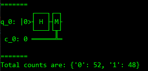
Sure enough we get approximately the same results we can expect by flipping a coin 100 times.
Pauli X example
Now let us demonstrate a Pauli X gate in action. With a similar setup as above, instead of passing the qubit through a Hadamard gate let us pass it through a Pauli X gate.
from qiskit import QuantumCircuit,execute,Aer
simulator = Aer.get_backend('qasm_simulator')
circuit = QuantumCircuit(1, 1)
# Add a Pauli X gate to qubit 0
circuit.x(0) # pylint: disable=no-member
circuit.measure([0], [0]) # pylint: disable=no-member
print(circuit)

job = execute(circuit, simulator, shots=100)
result = job.result()
counts = result.get_counts(circuit)
print("Total counts are:",counts) 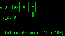
CNOT example
To implement a CNOT gate we will need to expand our circuit to have two qubits and two classical measurement bits. We will run the first qubit through a Hadamard gate to create a superposition state. We will then run that qubit through a CNOT gate as the control qubit with the second qubit, which is initialized as \(\left|0\right>\), as the target qubit of the gate.
circuit = QuantumCircuit(2, 2)
circuit.h(0) # pylint: disable=no-member
circuit.cx(0, 1) # pylint: disable=no-member
circuit.measure([0,1], [0,1]) # pylint: disable=no-member

print(circuit)
job = execute(circuit, simulator, shots=100)
result = job.result()

counts = result.get_counts(circuit)
print("Total counts are:",counts) 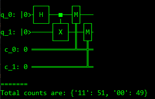
Based on the output of the run you may have noticed something interesting. With a qubit having been applied a Hadamard gate and the second qubit initialized as \(\left|0\right>\), the output is an initialized Bell state. We briefly touched on the topic in a previous section, however let us explore this a bit further. We know that a Bell state allows two or more qubits to become entangled. That means that if we were to measure one of the two qubits we should be able to gather information on the other qubit without having to measuring it.
It then becomes evident that if we run the same CNOT circuit as above and measure only one of the two qubits, we intrinsically know the value of the other. This is a simplified statement as there are more theoretical ramafications to this measurement, however I wanted to keep the scope of this article to the practical code.
Next Steps
The Bell state is important to understand as it forms the setup of many more advanced topics - more pointedly quantum cryptography. While I do not personally have enough understanding to tackle the topic currently, I do plan on continuing these studies and attempt to journey down the rabbit hole.
I plan on exploring and attempting to replicate Quantum Key Distribution - specifically the EE84 and E91 algorithms. While there are theoretical issues discussed surrounding the efficiency of QKD compared to the classical equivalents, I believe it is a natural next step to develop further quantum computing knowledge.
As always thanks folks, until next time!