
Introduction

In the culmination of what seemed like "Quantum February" I ended up participating in yet another quantum event - this time being run by the International Collegiate Programming Contest (ICPC) and hosted by IBM. Having participated in two other IBM ran events in the last year I was excited to jump back in and continue the journey to quantum learning.
The challenge consisted of three separate problems with smaller portions within the problem set. The first two challenges built off each other demonstrating how we can shift our thinking of the problem depending on the scope, while the third problem had us thinking of classic Boolean functions in quantum terms.
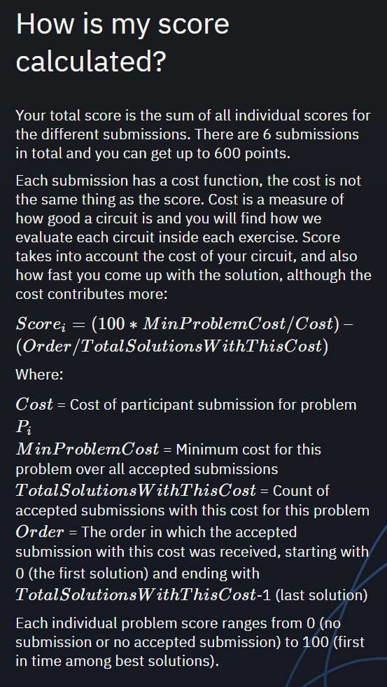
In standard IBM challenge methodology your final score is also largerly dependent on how efficient your circuits are while still solving the problem. A twist that was new in this event was not only efficiency of the circuit itself, but how quickly you were able to submit the initial solution. This lead to contestants finding themselves trying solve the challenges as quickly as possible, just to stake their claim to an initial solution position, and then spend the remaining time trying to refine their solutions. I'm still torn on whether I liked this particular nuance or not, however to the organizer's credit they did release the exact scoring formula after several participants asked for clarity. I will cover the scoring near the end of this post.
Without further ado, let us jump into the problems and my solutions.
Problem 1 - Popcount
The first notebook started off with a quick introduction of quantum circuits, gates, and Boolean functions in a quantum context. It reminded me quite a bit of going through IBM's Qiskit Textbook and helped set a baseline for participants who had not previously worked with Quantum Computing.
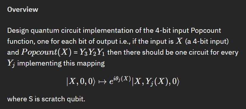
The problem statement starts off by covering a popular instruction - Popcount. Also known as Hamming weight the challenge notebook explains that hamming weight is leveraged in certain important quantum algorithms, such as Hamiltonian dymanics simulations, as they offer exponential advantage over classical solutions.
The challenge is to now implement our own popcount function using quantum circuits.
It took a few read throughs to understand exactly what we wanted to accomplish here. I was familiar enough with the concept of popcount however the challenge wording did trip me up at the beginning. The short version is that the first problem is implementing parts of the popcount function with 4 inputs.
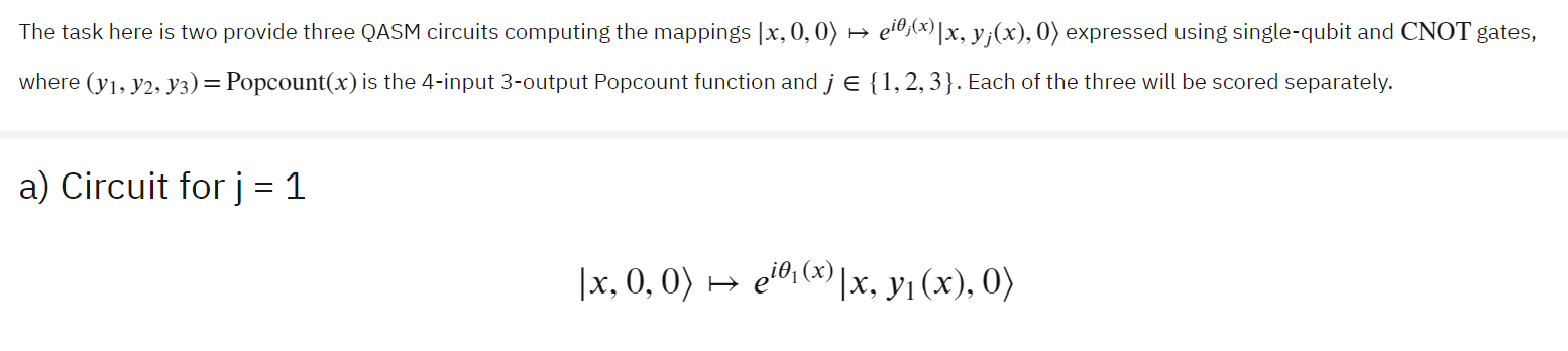
Problem 1.a
For this first 1.a portion - we are trying to encode how many 1's are in the least significant bit of the original input, essentially counting in binary. For an input of 0100, y1 = 1. For 1010, y1 = 0, etc...
Alright this doesn't seem too hard to account for, we should be able to leverage 4 CNOT gates, with each of our inputs acting as a control to our y1 output.
# Defining input, output and scratch qubits
x = 4    # number of input qubits
y1 = 1   # number of output qubit
s1 = 0   # number of scratch qubit

# Defining Quantum Circuit with the given circuits
def Circuit_1(In,Ou,Sc):

    # initiating required qubits
    X = QuantumRegister(In, 'input')
    Y= QuantumRegister(Ou, 'output')

    # creating circuit with above qubits
    Circ = QuantumCircuit(X,Y)

    ##### Create you circuit below #########

    Circ.cx(X[0], Y[0])
    Circ.cx(X[1], Y[0])
    Circ.cx(X[2], Y[0])
    Circ.cx(X[3], Y[0])

    ########################################

    # Transpiling the circuit into u, cnot
    Circ = transpile(Circ, basis_gates=['u3','cx'],optimization_level=3)

return Circ 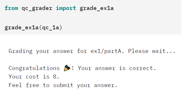
Problem 1.b
So far so good. The second part of the problem is to perform the same calculation, this time for the second LSB. This one ended up being the most complicated of the three parts of the first problem, mainly because there were more cases to take into consideration. After a bit of mulling over the approach, essentially what we needed to determine in an input = 4 situation is whether there were two or three inputs that were 1. The initial solution involved leveraging scratch qubits and essentially counting. This was an inneficient solution however, and I knew we could complete this without using any expensive, from a scoring perspective, scratch qubits. The improvement involved using a series of 6 Toffoli gates, coupling pairs of inputs, to determine whether only two or three of them were "on".
##### Create you circuit below #########

    Circ.ccx(X[0],X[1],Y[0])
    Circ.ccx(X[0],X[2],Y[0])
    Circ.ccx(X[0],X[3],Y[0])
    Circ.ccx(X[1],X[2],Y[0])
    Circ.ccx(X[1],X[3],Y[0])
    Circ.ccx(X[2],X[3],Y[0])
This was better, but there is still more I can do! Firstly, since we do not care about relative phase in this problem we can immediately gain some efficiency benefits by using RCCX gates instead of regular Toffoli. But that is not it either! If we take a closer look at the comparison groupings there seems to be quite a bit of rework. There were a few different things I started looking at. Firstly was ARXIV-0312225 which covers simplified Toffoli breakdowns. This essentially came down to the same complexity cost as an RCCX gate, so while interesting, did not get me much further. What really helped drive down the cost was when I broke down our RCCX gates and paired down the inneficient rework.
Using a subset to elaborate. If we break down two of our RCCX gates we get.
    #Circ.rccx(X[1],X[2],Y[0])
    Circ.ry(np.pi/4,Y[0])
    Circ.cx(X[2],Y[0])
    Circ.ry(np.pi/4,Y[0])
    Circ.cx(X[1],Y[0])
    Circ.ry(-np.pi/4,Y[0])
    Circ.cx(X[2],Y[0])
    Circ.ry(-np.pi/4,Y[0])

    #Circ.rccx(X[1],X[3],Y[0])
    Circ.ry(np.pi/4,Y[0])
    Circ.cx(X[3],Y[0])
    Circ.ry(np.pi/4,Y[0])
    Circ.cx(X[1],Y[0])
    Circ.ry(-np.pi/4,Y[0])
    Circ.cx(X[3],Y[0])
    Circ.ry(-np.pi/4,Y[0])
Do you see it yet? We are doing the same setup for both gate breakdowns. I can eliminate most of the second gate deconstruction by simply adding the Circ.cx(X[3],Y[0]) to the first breakdown - achieving the same end result.
    #Circ.rccx(X[1],X[2],Y[0])
    #Circ.rccx(X[1],X[3],Y[0])
    Circ.ry(np.pi/4,Y[0])
    Circ.cx(X[2],Y[0])
    Circ.cx(X[3],Y[0])
    Circ.ry(np.pi/4,Y[0])
    Circ.cx(X[1],Y[0])
    Circ.ry(-np.pi/4,Y[0])
    Circ.cx(X[3],Y[0])
    Circ.cx(X[2],Y[0])
    Circ.ry(-np.pi/4,Y[0])
With this knowledge I am able to combine three RCCX gates together and another two RCCX gates to a condensed version of our original circuit. The final structure then becomes the below.
def Circuit_2(In,Ou,Sc):
    if Sc != 0:
        # initiating required qubits
        X = QuantumRegister(In, 'input')
        Y = QuantumRegister(Ou, 'output')
        S = QuantumRegister(Sc, 'scratch')

        # creating circuit with above qubits
        Circ = QuantumCircuit(X,Y,S)
    else:

        # initiating required qubits
        X = QuantumRegister(In, 'input')
        Y= QuantumRegister(Ou, 'output')

        # creating circuit with above qubits
        Circ = QuantumCircuit(X,Y)

    ##### Create you circuit below #########

    #Circ.rccx(X[0],X[1],Y[0])
    #Circ.rccx(X[0],X[2],Y[0])
    #Circ.rccx(X[0],X[3],Y[0])
    Circ.ry(np.pi/4,Y[0])
    Circ.cx(X[1],Y[0])
    Circ.cx(X[2],Y[0])
    Circ.cx(X[3],Y[0])
    Circ.ry(np.pi/4,Y[0])
    Circ.cx(X[0],Y[0])
    Circ.ry(-np.pi/4,Y[0])
    Circ.cx(X[3],Y[0])
    Circ.cx(X[2],Y[0])
    Circ.cx(X[1],Y[0])
    Circ.ry(-np.pi/4,Y[0])

    #Circ.rccx(X[1],X[2],Y[0])
    #Circ.rccx(X[1],X[3],Y[0])
    Circ.ry(np.pi/4,Y[0])
    Circ.cx(X[2],Y[0])
    Circ.cx(X[3],Y[0])
    Circ.ry(np.pi/4,Y[0])
    Circ.cx(X[1],Y[0])
    Circ.ry(-np.pi/4,Y[0])
    Circ.cx(X[3],Y[0])
    Circ.cx(X[2],Y[0])
    Circ.ry(-np.pi/4,Y[0])

    #Circ.rccx(X[2],X[3],Y[0])
    Circ.ry(np.pi/4,Y[0])
    Circ.cx(X[3],Y[0])
    Circ.ry(np.pi/4,Y[0])
    Circ.cx(X[2],Y[0])
    Circ.ry(-np.pi/4,Y[0])
    Circ.cx(X[3],Y[0])
    Circ.ry(-np.pi/4,Y[0])

    ############################
    Circ = transpile(Circ, basis_gates=['u3','cx'],optimization_level=3)

return Circ 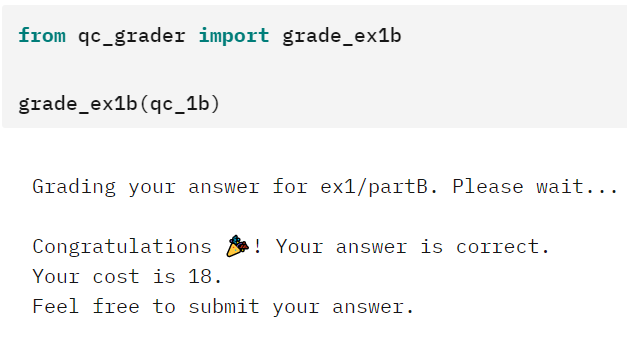
Problem 1.c
The third portion of this problem is to calculate our highest significant bit. With four inputs to consider our HSB can only be 1 if all inputs are also 1. Similarly to part b we do not need to take relative phase into consideration, therefore I can leverage RCCX gates instead of regular Toffolis and gain a bit of efficiency.
def Circuit_3(In,Ou,Sc):

    # initiating required qubits
    X = QuantumRegister(In, 'input')
    Y = QuantumRegister(Ou, 'output')

    # creating circuit with above qubits
    Circ = QuantumCircuit(X,Y)

    ##### Create you circuit below #########
    Circ.rccx(X[0],X[1],S[0])
    Circ.rccx(X[2],X[3],S[1])
    Circ.rccx(S[0],S[1],Y[0])
    Circ.rccx(X[0],X[1],S[0])
    Circ.rccx(X[2],X[3],S[1])

    ########################################

    # Transpiling the circuit into u, cnot
    Circ = transpile(Circ, basis_gates=['u3','cx'],optimization_level=3)

    return Circ
Problem 2 - Fourier Popcount
The second problem was essentially an extension of the first. While we were limited to 4 inputs on the first challenge, the second amped up the difficulty by having us consider a much larger 15 and 16 inputs. I could in theory leverage the same approach I did in the first problem, however the circuit complexity would quickly elevate if so. There has to be a more efficient method... and sure enough there is. After a bit of reading I got to ARXIV-1804.03719, more specifically using Quantum Fourier Transform (QFT) circuits.
Let's see how we can leverage this and solve the first 15-input problem.
Problem 2.a
We already know the popcount theory from our first theory. There will be 15 inputs, which means there can be at most 4 outputs - 1111 would represent 15 in binary, our largest possible number if all inputs were "on".
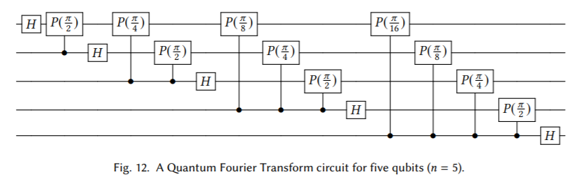
The Qiskit documentation on QFT provides a good intuition explanation on what I am was trying to achieve.
The quantum Fourier transform (QFT) transforms between two bases, the computational (Z) basis, and the Fourier basis. The H-gate is the single-qubit QFT, and it transforms between the Z-basis states |0⟩ and |1⟩ to the X-basis states |+⟩ and |−⟩. In the same way, all multi-qubit states in the computational basis have corresponding states in the Fourier basis. The QFT is simply the function that transforms between these bases.
Additionally, and more directly applicable when considering our problem statement, the Qiskit textbook provides a very elaborative set of GIFs on how counting works in QFT.
First in computational basis
Then in Fourier space
Since I will be using 15 inputs and 4 outputs the gifs essentially illustrate what I am trying to achieve. I think I'm almost able to put the approach to code now.
To leverage the QFT approach I need to setup the QFT, perform the rotations, and then perform the QFT-dagger to bring me back to original basis. Let's see if we can figure this out.
# Importing the qiskit module
from qiskit import *
import numpy as np
# Defining input, output and scratch qubits
x15 = 15 # number of input qubits
y15 = 4 # number of output qubit
s15 = 0 # number of scratch qubit
# Defining Quantum Circuit with the given circuits
def Circuit_15(In,Ou,Sc):
# initiating required qubits
X = QuantumRegister(In, 'input')
Y= QuantumRegister(Ou, 'output')
# creating circuit with above qubits
Circ = QuantumCircuit(X,Y)
##### Create you circuit below #########
#QFT
Circ.h(Y[0])
Circ.h(Y[1])
Circ.h(Y[2])
Circ.h(Y[3])
#Evaluate based on X0..X14
for i in range(15):
Circ.cp(np.pi/8, X[i], Y[3])
Circ.cp(np.pi/4, X[i], Y[2])
Circ.cp(np.pi/2, X[i], Y[1])
Circ.cp(np.pi, X[i], Y[0])
#Circ.barrier()
#QFT-Dagger
Circ.h(Y[0])
Circ.cp(-np.pi/2, Y[0], Y[1])
Circ.h(Y[1])
Circ.cp(-np.pi/4, Y[0], Y[2])
Circ.cp(-np.pi/2, Y[1], Y[2])
Circ.h(Y[2])
Circ.cp(-np.pi/8, Y[0], Y[3])
Circ.cp(-np.pi/4, Y[1], Y[3])
Circ.cp(-np.pi/2, Y[2], Y[3])
Circ.h(Y[3])
########################################
# Transpiling the circuit into u, cnot
Circ = transpile(Circ, basis_gates=['u3','cx'],optimization_level=3)
return Circ
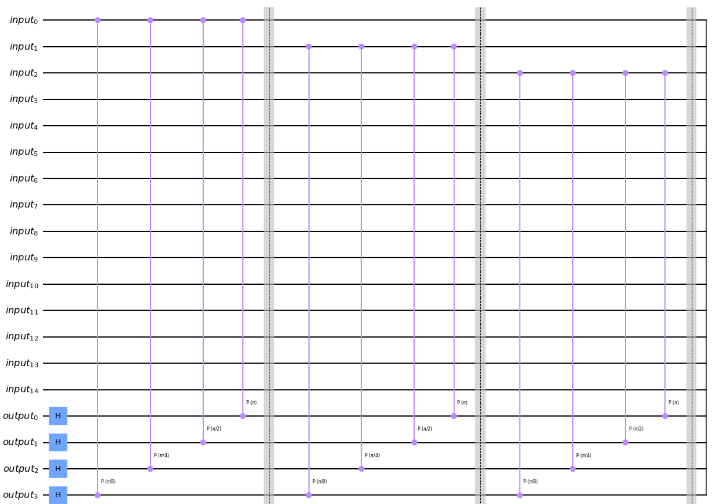
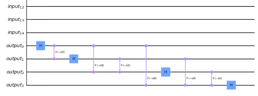
qc_2a = Circuit_15(x15,y15,s15)In this case since I know the outputs are starting at \(\left|0\right>\) I can partially cheat and shortcut the QFT portion by only using a Hadamard on them. Then rotate the outputs in Fourier basis, and bring it back to Computational basis with hopefully the right output.
A small section of the start and end of the circuit to drive home how the overall circuit looks like
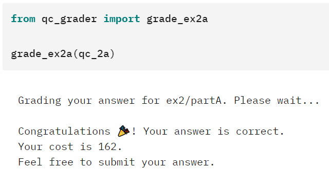
Thankfully after a few minor typos the grader returned some good news.
Problem 2.b
Are you sick of popcount yet? Hopefully not because we have one final problem related to it. This time, 16 inputs instead of 15. The big difference is if you remember that 15 can be represented as 1111, but 16 now must be represented by an additional output qubit - 10000. So 16 inputs, 5 outputs.
The main nuance is that we now need to go down to pi/16 for the fifth qubit. Everything else is the same as the first part of the challenge.
# Importing the qiskit module
from qiskit import *

# Defining input, output and scratch qubits
x16 =  16  # number of input qubits
y16 =  5  # number of output qubit
s16 =  0  # number of scratch qubit

# Defining Quantum Circuit with the given circuits
def Circuit_16(In,Ou,Sc):

    # initiating required qubits
    X = QuantumRegister(In, 'input')
    Y= QuantumRegister(Ou, 'output')
    # creating circuit with above qubits
    Circ = QuantumCircuit(X,Y)

    ##### Create you circuit below #########

    #QFT
    Circ.h(Y[0])
    Circ.h(Y[1])
    Circ.h(Y[2])
    Circ.h(Y[3])
    Circ.h(Y[4])
    #Evaluate based on X0..X15
    for i in range(16):
        Circ.cp(np.pi/16, X[i], Y[4])
        Circ.cp(np.pi/8, X[i], Y[3])
        Circ.cp(np.pi/4, X[i], Y[2])
        Circ.cp(np.pi/2, X[i], Y[1])
        Circ.cp(np.pi, X[i], Y[0])
    #QFT-Dagger
    Circ.h(Y[0])
    Circ.cp(-np.pi/2, Y[0], Y[1])
    Circ.h(Y[1])
    Circ.cp(-np.pi/4, Y[0], Y[2])
    Circ.cp(-np.pi/2, Y[1], Y[2])
    Circ.h(Y[2])
    Circ.cp(-np.pi/8, Y[0], Y[3])
    Circ.cp(-np.pi/4, Y[1], Y[3])
    Circ.cp(-np.pi/2, Y[2], Y[3])
    Circ.h(Y[3])
    Circ.cp(-np.pi/16, Y[0], Y[4])
    Circ.cp(-np.pi/8, Y[1], Y[4])
    Circ.cp(-np.pi/4, Y[2], Y[4])
    Circ.cp(-np.pi/2, Y[3], Y[4])
    Circ.h(Y[4])

    ########################################

    # Transpiling the circuit into u, cnot
    Circ = transpile(Circ, basis_gates=['u3','cx'],optimization_level=3)

    return Circ

qc_2b = Circuit_16(x16,y16,s16) 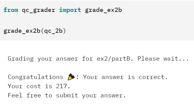
Just like that the second challenge is complete. Two down, one more to go!
Problem 3 - Unitaries
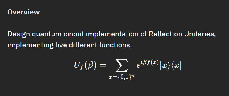
Shifting gears from leveraging popcount we now take a look at relative phase and how to compute Boolean functions into quantum states. Specifically:
In the previous two problems, the output of a classical Boolean function is computed into an additional qubit. However, quantum computers can also compute Boolean functions into the phase of a quantum state, which we explore in this problem.
In a more practical example the notebook covers what they actually mean by this. For a given function \(f(x_1 x_2) = x_1 x_2\) the Boolean function is "true" if and only iff both inputs are 1. For \(f(x_1 x_2) = x_1 + x_2\) the Boolean function is "true" only if either \(x_1\) or \(x_2\) are 1, but not both.
Our challenge is to create circuits that apply a relative phase to the our qubits when the circuit emulates a Boolean "true". The below illustrates the two sample functions in terms of quantum circuits and relative phase.
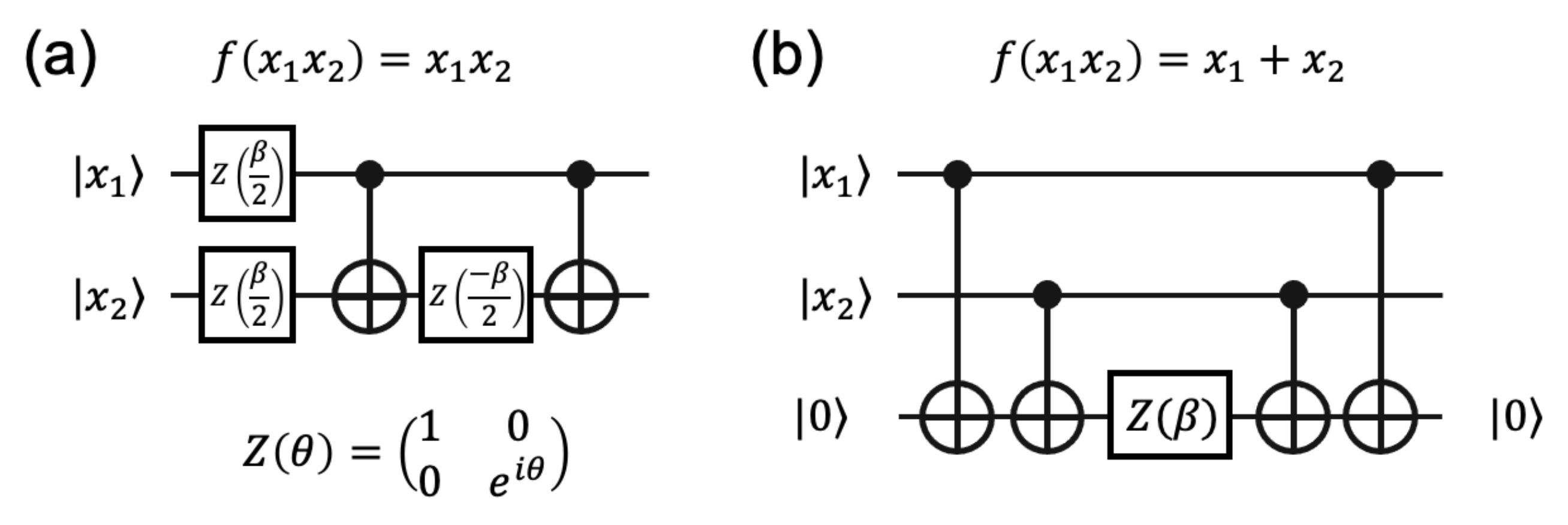
If we follow the logic of the circuit it becomes clear that on (a) a relative phase of β/2 is applied to both qubits, bringing us in line with a full β relative phase. As long as both qubits are 1 when the CNOTs flip \(x_2 \) the negative -β/2 phase doesn't get applied, leaving a full β relative phase on Boolean "true". It then becomes trivial to see that if either of the inputs are 0 the relative phase gets removed.
Similarly for (b) we can immediately see that with an auxiliary qubit starting as \(\left|0\right>\) if and only if a single input is 1 does the phase β get applied. Otherwise the CNOT gates put the aux qubit back to 0 and the phase is not applied.
With the background information clarified we are now presented with five different functions where we need to design the quantum circuit to add a relative phase when they "evaluate as true" in terms of the Boolean function.
Problem 3.a
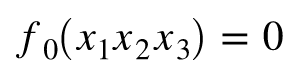
The first problem was the simplest but also maybe the one that took the most thinking to truly get. The Boolean function will never be true. Therefore it really doesn't matter what we do as a circuit since at no point there should be a relative phase added.
# Importing the qiskit module
from qiskit import *

q0 = 3   # number of required qubits
a0 = 0   # number of ancilla qubit
beta = circuit.Parameter('beta') #Parameter for reflection

# Defining Quantum Circuit with the given circuits
def Circuit_0(q,a,beta):
    # initiating required qubits
    Q = QuantumRegister(q, 'input')

    # creating circuit with above qubits
    Circ = QuantumCircuit(Q)

    ##### Create you circuit below #########
            # nothing!
    ########################################

    # Transpiling the circuit into u, cnot
    Circ = transpile(Circ, basis_gates=['u3','cx'],optimization_level=3)

    return Circ

qc_3a = Circuit_0(q0,a0,beta)
Problem 3.b
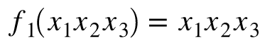
The second part of this problem becomes a Boolean true when all inputs are 1. There are several ways we can achieve this. Initially I went with two auxiliary qubits and leveraged RCCX with careful consideration that since RCCX doesn't play nice with relative phase to make sure to reverse it.
    Circ.rccx(Q[0],Q[1],A[1])
    Circ.rccx(Q[2],A[1],A[0])
    Circ.p(beta, A[0])
    Circ.rccx(Q[2],A[1],A[0])
    Circ.rccx(Q[0],Q[1],A[1])
Aux qubits are expensive however, so we can do better. Since it doesn't matter where we apply the relative phase, only that it is introduced we can consolidate the above and cut down one one qubit.
    Circ.rccx(Q[0], Q[1], A[0])
    Circ.cp(beta, A[0], Q[2])
    Circ.rccx(Q[0], Q[1], A[0])
We can still do better though! I wasn't aware of this Qiskit gate before this challenge but there is a nifty one-liner that achieves what we are trying to do, without any extra qubits! The MCP gate acts as a toffoli, applying a provided phase. Let's look at the full circuit now.
# Importing the qiskit module
from qiskit import *

q1 = 3  # number of required qubits
a1 = 0  # number of ancilla qubit
beta = circuit.Parameter('beta') #Parameter for reflection

# Defining Quantum Circuit with the given circuits
def Circuit_1(q,a,beta):

    # initiating required qubits
    Q = QuantumRegister(q, 'input')

     # creating circuit with above qubits
    Circ = QuantumCircuit(Q)

    ##### Create you circuit below #########

    Circ.mcp(beta, [Q[0], Q[1]], Q[2])

    ########################################

    return Circ

qc_3b = Circuit_1(q1,a1,beta)
Problem 3.c

For this portion of the problem all the inputs need to either be 1 or 0. When they are all 1 the left portion \(x_1 x_2 x_3\) evaluates as 1 while the right portion \((1-x_1)(1-x_2)(1-x_3)\) becomes 0, meaning it evaluates as 1+0. When the inputs are all 0 the inverse happens. At any point where there is a mix of inputs that are 1 and 0 the overall term becomes 0. Using our same MCP gate from above we can codify this easily enough.
# Importing the qiskit module
from qiskit import *
q2 = 3 # number of required qubits
a2 = 0 # number of ancilla qubit
beta = circuit.Parameter('beta') #Parameter for reflection
# Defining Quantum Circuit with the given circuits
def Circuit_2(q,a,beta):
# initiating required qubits
Q = QuantumRegister(q, 'input')
# creating circuit with above qubits
Circ = QuantumCircuit(Q)
##### Create you circuit below #########|
#assuming 111
#Circ.rccx(Q[0], Q[1], A[0])
#Circ.cp(beta, A[0], Q[2])
#Circ.rccx(Q[0], Q[1], A[0])
Circ.mcp(beta, [Q[0], Q[1]], Q[2])
#assuming 000
Circ.x(Q[0])
Circ.x(Q[1])
Circ.x(Q[2])
#Circ.rccx(Q[0], Q[1], A[0])
#Circ.cp(beta, A[0], Q[2])
#Circ.rccx(Q[0], Q[1], A[0])
Circ.mcp(beta, [Q[0], Q[1]], Q[2])
Circ.x(Q[0])
Circ.x(Q[1])
Circ.x(Q[2])
########################################
# Transpiling the circuit into u, cnot
Circ = transpile(Circ, basis_gates=['u3','cx'],optimization_level=3)
return Circ
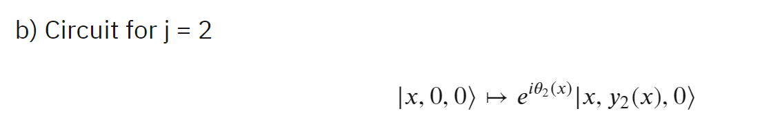
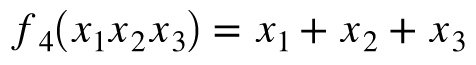
qc_3c = Circuit_2(q2,a2,beta)Problem 3.d
This would be what I consider the most challenging of the third problem components conceptually. In this case the function becomes a Boolean true if and only if a single input is 1 - which matches up with having three possible solutions. Let me start with using the single qubit phase application portion of the circuit.
    for i in range(q3):
        Circ.cx(Q[i], A[0])
    Circ.p(beta, A[0])
    for i in reversed(range(q3)):
Circ.cx(Q[i], A[0]) 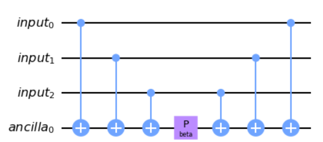
You can follow along and see that when a single input is 1, phase gets applied. When two are 1 the phase does not get applied. But if all three are enabled we still get the phase applied. So we need to take care of this particular edge case as well. I can add an negative β leveraging our MCP gate so it eliminates this scenario from the overall circuit. The full circuit ends up being.
# Importing the qiskit module
from qiskit import *
import numpy as np

q3 = 3  # number of required qubits
a3 = 1  # number of ancilla qubit
beta = circuit.Parameter('beta') #Parameter for reflection

# Defining Quantum Circuit with the given circuits
def Circuit_3(q,a,beta):

    # initiating required and ancilla qubits
    Q = QuantumRegister(q, 'input')
    A = QuantumRegister(a, 'ancilla')

    # creating circuit with above qubits
    Circ = QuantumCircuit(Q,A)

    ##### Create you circuit below #########

    #Circ.rccx(Q[0], Q[1], A[0])
    #Circ.cp(-beta, A[0], Q[2])
    #Circ.rccx(Q[0], Q[1], A[0])
    Circ.mcp(-beta, [Q[0], Q[1]], Q[2])

    for i in range(q3):
        Circ.cx(Q[i], A[0])
    Circ.p(beta, A[0])
    for i in reversed(range(q3)):
        Circ.cx(Q[i], A[0])

    ########################################

    # Transpiling the circuit into u, cnot
    Circ = transpile(Circ, basis_gates=['u3','cx'],optimization_level=3)

    return Circ

qc_3d = Circuit_3(q3,a3,beta) 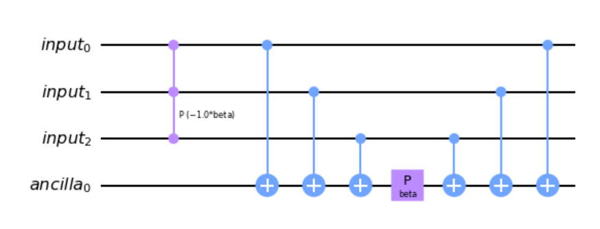
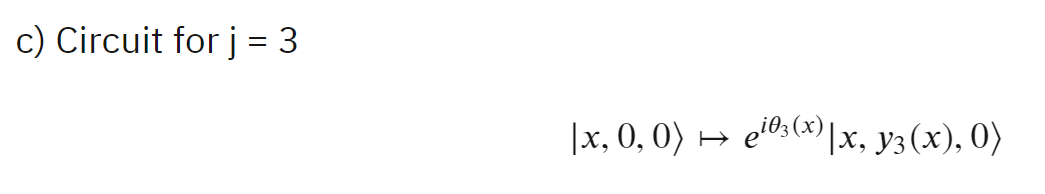
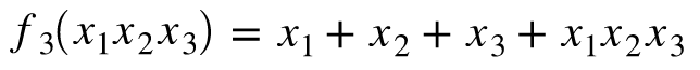
Problem 3.e
The last part of the problem! This one actually ends up being a simplified portion of the previous part - with a caveat. I couldn't understand at first HOW there were 4 solutions for the equation \(x_1 + x_2 + x_3\) until I realized that we are essentially wrapping the count. So the solution is if only one of the three qubits are 1, which accounts for three solutions, but we have one more. When all three inputs are 1 we can essentially consider the Boolean output as 1, or true, as well. This ends up being the same solution as our previous part, without the MCP to account for the condition where all inputs are 1.
# Importing the qiskit module
from qiskit import *
q4 = 3 # number of required qubits
a4 = 1 # number of ancilla qubit
beta = circuit.Parameter('beta') #Parameter for reflection
# Defining Quantum Circuit with the given circuits
def Circuit_4(q, a, beta):
# initiating required and ancilla qubits
Q = QuantumRegister(q, 'input')
A = QuantumRegister(a, 'ancilla')
# creating circuit with above qubits
Circ = QuantumCircuit(Q,A)
##### Create you circuit below #########
Circ.cx(Q[0],A[0])
Circ.cx(Q[1],A[0])
Circ.cx(Q[2],A[0])
Circ.p(beta, A[0])
Circ.cx(Q[2],A[0])
Circ.cx(Q[1],A[0])
Circ.cx(Q[0],A[0])
########################################
# Transpiling the circuit into u, cnot
Circ = transpile(Circ, basis_gates=['u3','cx'],optimization_level=3)
return Circ
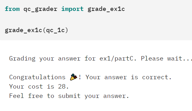
qc_3e = Circuit_4(q4,a4,beta)With that I can run the solutions through the grader and see where this ends up.
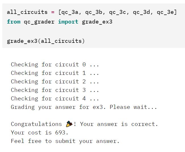
Conclusion & Recap
The scoring for this event was interesting in that it also took into consideration when you initially submitted a successful answer. There were quite a few questions from the participants as to how this worked and during the competition the ICPC and IBM teams released a good breakdown on the calculation.
I will be honest and wish this would have been clearer from the beginning. I was only able to start the challenges on Saturday, despite the event starting Thursday and potentially lost some valuable points due to the delayed start. Ultimately I am happy that the team responded to the participants and did add the the scoring algorithm to clarify how it was being judged.
Another nuance, which did not get a clear answer that I am aware of, is that throughout the challenge invalid answers were stripped from the leaderboards. Answers falling outside the bounds of the challenge, such as issuing resets mid circuit, were removed and the score eliminated. Now this opens the question of whether the "order of successful answer" also gets reset with this these eliminations. On one side I believe they should be removed as the answer was not deemed valid, however on the other hand there are two points - first that it was not explicitly stated that these approaches would not be valid/the grader allowed them through, and secondly that there was no way to submit a "worst" answer once the invalid, more efficient solution was submitted. Food for thought but I felt this could have been a bit more transparent.
Once everything was said, done and the submission portal was closed, there was a period of a couple weeks where the ICPC team went through the top submissions to ensure they conformed to the spirit of the competition. Once that was done I am happy to say that I squared out the top 20 of overall submissions.

As with all the IBM based events I came out of it learning much more than what I came into the event with. Additionally this was the first event where tips and tricks from previous events (such as the RCCX decomposition) were carried over and applied. Clearly it looks like at least something is sticking by doing these events! Honestly it was a really well run event and I thank the ICPC and IBM teams for organizing and running it. I managed to knock off a few more positions in the global standings and hoping to see myself crack the top 10 in upcoming events.

Thanks folks, until next time!