Qiskit Quantum Challenge - Africa 2021

Introduction

I do not think I can give a better introduction to this challenge than the verbiage on the first notebook:

Quantum Computing has the potential to revolutionize computing, as it can solve problems that are not possible to solve on a classical computer. This extra ability that quantum computers have is called quantum advantage. To achieve this goal, the world needs passionate and competent end-users: those who know how to apply the technology to their field.

In this challenge you will be exposed, at a high-level, to quantum computing through Qiskit. As current or future users of quantum computers, you need to know what problems are appropriate for quantum computation, how to structure the problem model/inputs so that they are compatible with your chosen algorithm, and how to execute a given algorithm and quantum solution to solve the problem.

Preparing for a quantum future starts now. By learning how to model and apply our current problems prepares us to tackle future issues which we may not even be aware of yet. Each and every of these challenges is another stepping stone in our journey of quantum learning.

With that said, let us dive into the challenges!

Crop Yield

Our first challenge tasks us with finding optimal crop distributions given a set of land and types of crops we can plant. The goal is to maximize our food output. What we will soon learn is that this type of problem can be modelled as a Quadratic equation, and the minimum of the equation will not only give us the most efficient food output, but this type of problem is something that Quantum computers excel at doing.

Quadratic Equation Model

Let us start off with how a quadratic equation looks like with an example and constraints.

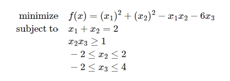
The next step is to convert it to usable code. Qiskit has a useful QuadraticProgram module that allows us to do just that.

quadprog = QuadraticProgram(name="example 1")
quadprog.integer_var(name="x_1", lowerbound=0, upperbound=4)
quadprog.integer_var(name="x_2", lowerbound=-2, upperbound=2)
quadprog.integer_var(name="x_3", lowerbound=-2, upperbound=4)
quadprog.minimize(
    linear={"x_3": -6},
    quadratic={("x_1", "x_1"): 1, ("x_2", "x_2"): 1, ("x_1", "x_2"): -1},
)
quadprog.linear_constraint(linear={"x_1": 1, "x_2": 1}, sense="=", rhs=2)
quadprog.quadratic_constraint(quadratic={("x_2", "x_3"): 1}, sense=">=", rhs=1)

Then if we print out the Linear Programming string we can confirm that it looks right.

print(quadprog.export_as_lp_string())

\ This file has been generated by DOcplex
\ ENCODING=ISO-8859-1
\Problem name: example 1

Minimize
 obj: - 6 x_3 + [ 2 x_1^2 - 2 x_1*x_2 + 2 x_2^2 ]/2
Subject To
 c0: x_1 + x_2 = 2
 q0: [ x_2*x_3 ] >= 1

Bounds
       x_1 <= 4
 -2 <= x_2 <= 2
 -2 <= x_3 <= 4

Generals
 x_1 x_2 x_3
End

That does indeed look right based on our example. Time to see if we can use this knowledge and apply it to the crop yield challenge!

Crop Yield Application

We are given a problem set of 3 hectares of land and various constraints on the crops we can grow.

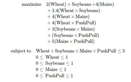
We can then take the same approach as the example and model this to code we can use with a quantum computer.

def cropyield_quadratic_program():
    cropyield = QuadraticProgram(name="Crop Yield")
    ##############################
    # Put your implementation here
    # Setting integers and bounds 
    cropyield.integer_var(name="Wheat", lowerbound=0, upperbound=1)
    cropyield.integer_var(name="Soybeans", lowerbound=0, upperbound=1)
    cropyield.integer_var(name="Maize", lowerbound=0, upperbound=1)
    cropyield.integer_var(name="PushPull", lowerbound=0, upperbound=1)

    # Set the quadratic to maximize
    cropyield.maximize(
        linear={"Wheat": 2,"Soybeans": 1,"Maize": 4},
        quadratic={("Wheat", "Soybeans"): 2.4, ("Wheat", "Maize"): 4, ("Wheat", "PushPull"): 4, 
                   ("Soybeans", "Maize"): 2, ("Soybeans", "PushPull"): 1, ("Maize", "PushPull"): 5},
    )
    
    cropyield.linear_constraint(linear={"Wheat": 1, "Soybeans": 1,"Maize": 1, "PushPull": 1}, sense="<=", rhs=3)
    ##############################
    return cropyield

Classical Solution

We shall solve the equation three separate ways - the first avoiding the quantum world and using a classic Numpy approach.

def get_classical_solution_for(quadprog: QuadraticProgram):
    # Create solver
    solver = NumPyMinimumEigensolver()

    # Create optimizer for solver
    optimizer = MinimumEigenOptimizer(solver)

    # Return result from optimizer
    return optimizer.solve(quadprog)

Solution found using the classical method:

Maximum crop-yield is 19.0 tons
Crops used are: 
      1.0 ha of Wheat
      0.0 ha of Soybeans
      1.0 ha of Maize
      1.0 ha of PushPull

And with that we have a baseline to work with. Let’s repeat the solution using two quantum methods.

VQE Solution

The first quantum approach we will explore is the Variational Quantum Eigensolver algorithm, or VQE. The algorithm uses a variational technique to find the minimum eigenvalue of the Hamiltonian 𝐻 of a given system.

An instance of VQE requires defining two algorithmic sub-components: a trial state (ansatz) which is a QuantumCircuit, and one of the classical optimizers. The ansatz is varied, via its set of parameters, by the optimizer, such that it works towards a state, as determined by the parameters applied to the ansatz, that will result in the minimum expectation value being measured of the input operator (Hamiltonian).

def get_VQE_solution_for(quadprog: QuadraticProgram, quantumInstance: QuantumInstance, optimizer=None,):

    # Create solver and optimizer
    solver = VQE(optimizer=optimizer, quantum_instance=quantumInstance, callback=callback)

    # Create optimizer for solver
    optimizer = MinimumEigenOptimizer(solver)

    # Get result from optimizer
    result = optimizer.solve(quadprog)
    return result, _eval_count

Solution found using the VQE method:

Maximum crop-yield is 19.0 tons
Crops used are: 
      1.0 ha of Wheat
      0.0 ha of Soybeans
      1.0 ha of Maize
      1.0 ha of PushPull

The solution was found within 25 evaluations of VQE

QAOA Solution

The second quantum solution we will explore is the Quantum Approximate Optimization Algorithm, or QAOA.

The QAOA implementation directly extends VQE and inherits VQE’s optimization structure. However, unlike VQE, which can be configured with arbitrary ansatzes, QAOA uses its own fine-tuned ansatz, which comprises 𝑝 parameterized global 𝑥 rotations and 𝑝 different parameterizations of the problem hamiltonian. QAOA is thus principally configured by the single integer parameter, p, which dictates the depth of the ansatz, and thus affects the approximation quality.

Let’s apply it and see if it not only finds the same solution, but if the fine-tuned ansatz also allows us to reduce the amount of evaluations required.

def get_QAOA_solution_for(quadprog: QuadraticProgram, quantumInstance: QuantumInstance, optimizer=None,):

    # Create solver
    solver = QAOA(optimizer=optimizer, quantum_instance=quantumInstance, callback=callback,)

    # Create optimizer for solver
    optimizer = MinimumEigenOptimizer(solver)

    # Get result from optimizer
    result = optimizer.solve(quadprog)
    return result, _eval_count

Solution found using the QAOA method:

Maximum crop-yield is 19.0 tons
Crops used are: 
      1.0 ha of Wheat
      0.0 ha of Soybeans
      1.0 ha of Maize
      1.0 ha of PushPull

The solution was found within 3 evaluations of QAOA.

Portfolio Optimization

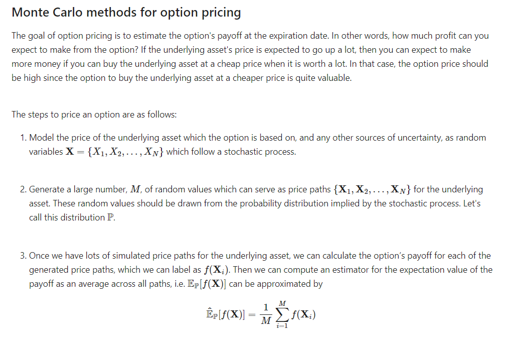
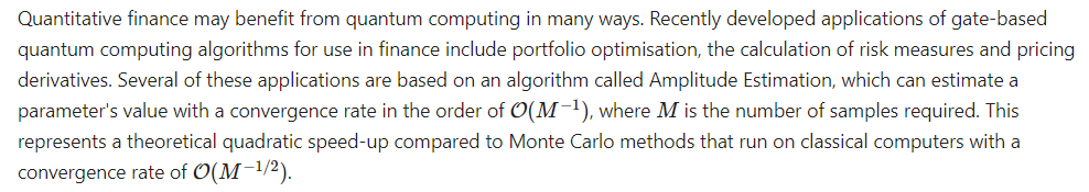
The second of the problems in this challenge revolves around exploring a Monte Carlo sampling to help valuate Options pricing. It has been shown that when applying these techniques to quantum computers we are able to achieve a quadratic speedup in comparison to the classical approach.

Our challenge can be broken down into three steps:

Let’s use a classical approach first to show how it works in action.

Classical Solution

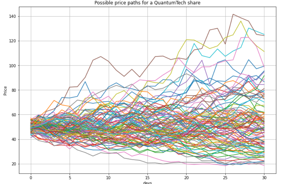
Using a fictitious QuantumTech share, we were tasked with filling in the appropriate details. We are essentially creating many possible realities, then computing the average.

A Monte Carlo approach simply samples random values for the parameters of your function from an underlying distribution and computes the function multiple times, each time using a different set of randomly sampled values. In doing so, we can obtain an expected value for the function we are trying to evaluate by taking an average over all the computed values of the function

# Monte Carlo valuation of a European call option 

# set a random seed to reproduce our results
np.random.seed(42)

# set the parameters
S0 = 50 # initial price of the underlying asset
K = 55 # strike price
r = 0.05 # average return of the underlying
sigma = 0.4 # volatility of the underlying
T = 1 # time till execution
t = 30 # number of time steps we want to divide T in
dt = T / t # incremental time step size
M = 1000 # number of paths to simulate

# Simulating M price paths with t time steps
# sum instead of cumsum would also do if only the final values at end of the month (i.e. at time T) are of interest
S = S0 * np.exp(np.cumsum((r - 0.5 * sigma ** 2) * dt + sigma * math.sqrt(dt)* np.random.standard_normal((t + 1, M)), axis=0))

# Calculating the Monte Carlo estimator for the expected payoff
P_call = sum(np.maximum(S[-1] - K, 0)) / M

# Results output
print("The call option value is:  {:0.2f} ZAR.\n".format(P_call))

Which when executed, the simple example returns us a target price.

The call option value is:  7.64 ZAR.

While we have the average, let’s look at the distribution of the various “realities” we created as part of the Monte Carlo approach.

Alright we have a good grasp on how this looks like classically. Let’s take a look at the quantum approach and how we can get a quadratic speedup.

Quantum Solution

To convert our classical approach to a quantum one we would need to perform three steps.

• Represent the probability distribution P describing the evolution of the share price of QuantumTech on a quantum computer.
• Construct the quantum model which computes the payoff of the option,f(X).
• Calculate the expectation value of the payoff Ep[f(X)]

Quantum Uncertainty Model

Returning to our QuantumTech example, the first component of our option pricing model is to create a quantum circuit that takes in the probability distribution implied.

# number of qubits to represent the uncertainty/distribution
num_uncertainty_qubits = 2

# parameters for considered random distribution
S = 50       # initial spot price
strike_price = 55
vol = 0.4     # volatility of 40%
r = 0.05      # annual interest rate of 5%
T = 30 / 365  # 30 days to maturity

# resulting parameters for log-normal distribution
mu = ((r - 0.5 * vol**2) * T + np.log(S))
sigma = vol * np.sqrt(T)
mean = np.exp(mu + sigma**2/2)
variance = (np.exp(sigma**2) - 1) * np.exp(2*mu + sigma**2)
stddev = np.sqrt(variance)

# lowest and highest value considered for the spot price; in between, an equidistant discretization is considered.
# we truncate the distribution to the interval defined by 2 standard deviations around the mean
low  = np.maximum(0, mean - 2*stddev) 
high = mean + 2*stddev

# construct circuit factory for uncertainty model
uncertainty_model = LogNormalDistribution(num_uncertainty_qubits, mu=mu, sigma=sigma**2, bounds=(low, high))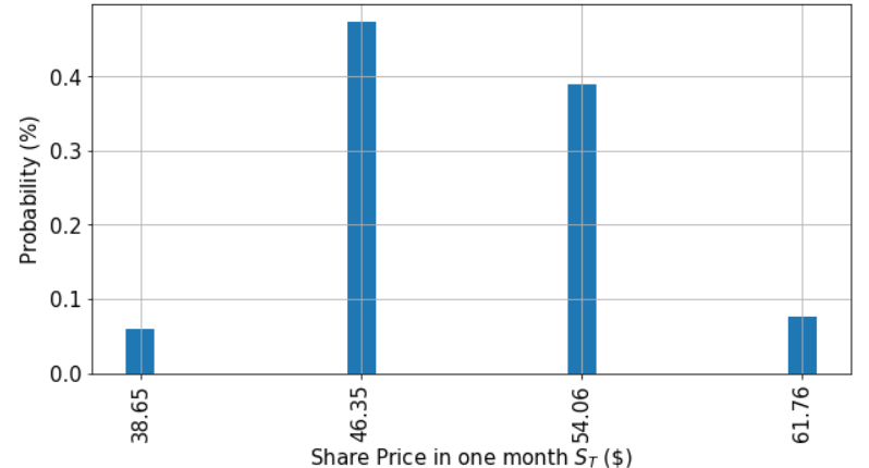

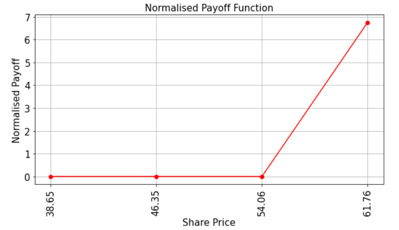
Payoff Function

Let’s have a look at the payoff function for our QuantumTech option. Recall that the payoff function equals zero as long as the share price in 1 months time, St, is less than the strike price K and then increases linearly thereafter. The code below illustrates this.

Evaluate Expected Payoff

Lastly, we can use Quantum Amplitude Estimation to compute the expected payoff of the option. Qiskit has a built-in module, EuropeanCallPricing which we can leverage to make this happen.

from qiskit_finance.applications.estimation import EuropeanCallPricing

european_call_pricing = EuropeanCallPricing(num_state_qubits=num_uncertainty_qubits,
                                            strike_price=strike_price,
                                            rescaling_factor=0.25,
                                            bounds=(low, high),
                                            uncertainty_model=uncertainty_model)

# evaluate exact expected value (normalized to the [0, 1] interval)
exact_value = np.dot(uncertainty_model.probabilities, y)

conf_int = np.array(result.confidence_interval_processed)
print('Exact value:        \t%.4f' % exact_value)
print('Estimated value:    \t%.4f' % (european_call_pricing.interpret(result)))
print('Estimation error:    \t%.4f' %(np.abs(exact_value-european_call_pricing.interpret(result))))
print('Confidence interval:\t[%.4f, %.4f]' % tuple(conf_int))

Exact value:        	0.5199
Estimated value:    	0.4985
Estimation error:    	0.0214
Confidence interval:	[-0.4018, 1.3988]

One of the challenge components of this notebook was also to find a more accurate representation than above. While we saw how to implement the overall process, we ideally would want to reduce the error as much as possible and have our estimated values as close to the exact values as we can.

By tweaking the various variables we are able to accomplish just that.

num_uncertainty_qubits = 2
low  = np.maximum(0, mean - 2*stddev) 
high = mean + 2*stddev
epsilon = 0.08
alpha = 0.06
shots = 10
simulator = 'qasm_simulator'

# Run this cell once you are ready to submit your answer

from qc_grader import grade_ex2a
solutions = [num_uncertainty_qubits, low, high, epsilon, alpha, shots, simulator]
grade_ex2a(solutions)

Quantum Chemistry

Quantum computing promises spectacular improvements in drug-design. In particular, in order to design new anti-retrovirals it is important to perform chemical simulations to confirm that the anti-retroviral binds with the virus protein. Such simulations are notoriously hard and sometimes ineffective on classical supercomputers. Quantum computers promise more accurate simulations allowing for a better drug-design workflow.

In this challenge we will explore the VQE approach more in-depth and attempt to see whether our toy anti-retroviral molecule binds with a toy virus.

Define Protease/Anti-Retroviral

We are given the toy Protease to use in our challenge.

We are also given our toy Anti-Retroviral. These two items will be used in the next steps where our goal is to see if we are able to bond both of them.

Model the Macro Molecule

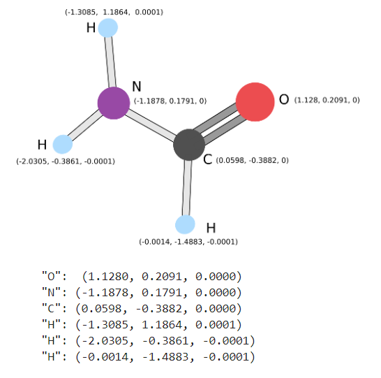
Now that we know what our Macro Molecule should look like, we can use the previous examples in the notebook to help model our new one. In theory we should be able to add on the Anti-Retroviral, which should just be the Carbon, to the existing model we had for the Protease.

molecular_variation = Molecule.absolute_stretching

specific_molecular_variation = apply_variation_to_atom_pair(molecular_variation, atom_pair=(6, 1))

macromolecule = Molecule(geometry=
                             [['O', [1.1280, 0.2091, 0.0000]],
                              ['N', [-1.1878, 0.1791, 0.0000]],
                              ['C', [0.0598, -0.3882, 0.0000]],
                              ['H', [-1.3085, 1.1864, 0.0001]],
                              ['H', [-2.0305, -0.3861, -0.0001]],
                              ['H', [-0.0014, -1.4883, -0.0001]],
                              ['C', [-0.1805, 1.3955, 0.0000]]],
                             charge=0, multiplicity=1, degrees_of_freedom=[specific_molecular_variation])

#"O":  (1.1280, 0.2091, 0.0000)
#"N": (-1.1878, 0.1791, 0.0000)
#"C": (0.0598, -0.3882, 0.0000)
#"H": (-1.3085, 1.1864, 0.0001)
#"H": (-2.0305, -0.3861, -0.0001)
#"H": (-0.0014, -1.4883, -0.0001)

Energy Landscape - Does It Bind?

Following the example earlier in the notebook we can model up the binding interaction and plot out the energy landscape to see if our toy example binds.

def construct_hamiltonian_solve_ground_state(
    molecule,
    num_electrons=2,
    num_molecular_orbitals=2,
    chemistry_inspired=True,
    hardware_inspired_trial=None,
    vqe=True,
    perturbation_steps=np.linspace(-1, 1, 3),
):
    """Creates fermionic Hamiltonion and solves for the energy surface.

    Args:
        molecule (Union[qiskit_nature.drivers.molecule.Molecule, NoneType]): The molecule to simulate.
        num_electrons (int, optional): Number of electrons for the `ActiveSpaceTransformer`. Defaults to 2.
        num_molecular_orbitals (int, optional): Number of electron orbitals for the `ActiveSpaceTransformer`. Defaults to 2.
        chemistry_inspired (bool, optional): Whether to create a chemistry inspired trial state. `hardware_inspired_trial` must be `None` when used. Defaults to True.
        hardware_inspired_trial (QuantumCircuit, optional): The hardware inspired trial state to use. `chemistry_inspired` must be False when used. Defaults to None.
        vqe (bool, optional): Whether to use VQE to calculate the energy surface. Uses `NumPyMinimumEigensolver if False. Defaults to True.
        perturbation_steps (Union(list,numpy.ndarray), optional): The points along the degrees of freedom to evaluate, in this case a distance in angstroms. Defaults to np.linspace(-1, 1, 3).

    Raises:
        RuntimeError: `chemistry_inspired` and `hardware_inspired_trial` cannot be used together. Either `chemistry_inspired` is False or `hardware_inspired_trial` is `None`.

    Returns:
        qiskit_nature.results.BOPESSamplerResult: The surface energy as a BOPESSamplerResult object.
    """
    # Verify that `chemistry_inspired` and `hardware_inspired_trial` do not conflict
    if chemistry_inspired and hardware_inspired_trial is not None:
        raise RuntimeError(
            (
                "chemistry_inspired and hardware_inspired_trial"
                " cannot both be set. Either chemistry_inspired"
                " must be False or hardware_inspired_trial must be none."
            )
        )

    # Step 1 including refinement, passed in

    # Step 2a
    molecular_orbital_maker = PySCFDriver(
        molecule=molecule, unit=UnitsType.ANGSTROM, basis="sto3g"
    )

    # Refinement to Step 2a
    split_into_classical_and_quantum = ActiveSpaceTransformer(
        num_electrons=num_electrons, num_molecular_orbitals=num_molecular_orbitals
    )

    fermionic_hamiltonian = ElectronicStructureProblem(
        molecular_orbital_maker, [split_into_classical_and_quantum]
    )
    fermionic_hamiltonian.second_q_ops()

    # Step 2b
    map_fermions_to_qubits = QubitConverter(JordanWignerMapper())

    # Step 3a
    if chemistry_inspired:
        molecule_info = fermionic_hamiltonian.molecule_data_transformed
        num_molecular_orbitals = molecule_info.num_molecular_orbitals
        num_spin_orbitals = 2 * num_molecular_orbitals
        num_electrons_spin_up_spin_down = (
            molecule_info.num_alpha,
            molecule_info.num_beta,
        )
        initial_state = HartreeFock(
            num_spin_orbitals, num_electrons_spin_up_spin_down, map_fermions_to_qubits
        )

        chemistry_inspired_trial = UCCSD(
            map_fermions_to_qubits,
            num_electrons_spin_up_spin_down,
            num_spin_orbitals,
            initial_state=initial_state,
        )

        trial_state = chemistry_inspired_trial
    else:
        if hardware_inspired_trial is None:
            hardware_inspired_trial = TwoLocal(
                rotation_blocks=["ry"],
                entanglement_blocks="cz",
                entanglement="linear",
                reps=2,
            )

        trial_state = hardware_inspired_trial

    # Step 3b and alternative
    if vqe:
        noise_free_quantum_environment = QuantumInstance(Aer.get_backend('statevector_simulator'))
        solver = VQE(ansatz=trial_state, quantum_instance=noise_free_quantum_environment)
    else:
        solver = NumPyMinimumEigensolver()

    # Step 4 and alternative
    ground_state = GroundStateEigensolver(map_fermions_to_qubits, solver)

    # Refinement to Step 4
    energy_surface = BOPESSampler(gss=ground_state, bootstrap=False)
    energy_surface_result = energy_surface.sample(
        fermionic_hamiltonian, perturbation_steps
    )

    return energy_surface_result

With the structure setup, we can then execute and graph it out.

q1_energy_surface_result = construct_hamiltonian_solve_ground_state(
    molecule=macromolecule,
    num_electrons=2,
    num_molecular_orbitals=2,
    chemistry_inspired=True,
    vqe=True,
    perturbation_steps=np.linspace(-0.5, 5, 30),
)

plot_energy_landscape(q1_energy_surface_result)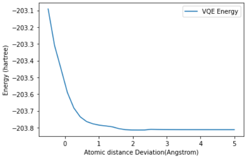

The last question we needed to answer was whether this interaction bonded or not. Sadly, based on the energy landscape graph we have to answer:

D. No, there is no clear minimum for any separation, so there is no binding.

While this wasn’t a great ending for our toy Anti-Retroviral, it at least shows us how we can structure such problems in a quantum space, and just how much of an impact a speedup in this space could result in.

Conclusion

As usual, I left this event having learned much more than I started it with. Even though I don’t fancy myself a future virologist learning how a space like Quantum Computing could intersect with other fields, and just how important it is that we are talking to one another and cross polinating our specific areas of focus. When we all work together, building upon one another, we will move the collective human needle forward. I’m excited for my small part in that journey so far, and I cannot wait to see where it takes me.

As always thanks folks, until next time!