Qiskit Quantum Challenge - Fall 2021

Introduction

The IBM Fall 2021 Quantum challenge presented us with yet another exciting opportunity to explore quantum computing in our world today. Leveraging the latest Qiskit capabilities available, this challenge stood out to me by allowing us to explore essentially real-world scenarios. Optimizing portfolio distributions, image classification processes, and optimal revenue scheduling are situations that mentally move me further away from theoretical quantum computing, and more into “solving everyday problems using quantum computing”. Just as I had a turning point when I started my journey with Qiskit back 2019, where it moved from mathematical theory to application in code, I felt with this event that I was moving away from simply applying the theory in code to practically solving real problems.

With that said, let’s dive into a few of the challenges and go over how I approached solving them!

Portfolio Optimization

The challenge statement starts out as:

The goal of this exercise is to find the efficient frontier for an inherent risk using a quantum approach. We will use Qiskit's Finance application modules to convert our portfolio optimization problem into a quadratic program so we can then use variational quantum algorithms such as VQE and QAOA to solve our optimization problem

While we have covered Variational Quantum Eigensolver (VQE) and Quantum Approximate Optimization Algorithm (QAOA) and how to leverage them in previous challenges, we need to cover what an efficient frontier and understand how that ties into the overall situation.

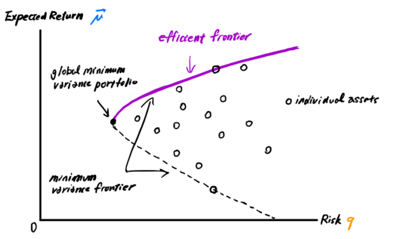
The challenge notebook goes on to explain Modern Portfolio Theory and how we apply it in our situation. What we are looking to accomplish is a maximal return based on portfolio holdings. The minimum variance frontier shows the minimum variance that can be achieved for a given level of expected return. By holding a portfolio below this point, we will always get a higher return along the positive slop of the frontier - also called the efficient frontier.

So how do we get started? The function which describes the efficient frontier can be formulated into a quadratic program with linear constraints. Before even seeing the formula we can start to see where the VQE/QAOA implementation will help with the quadratic function.

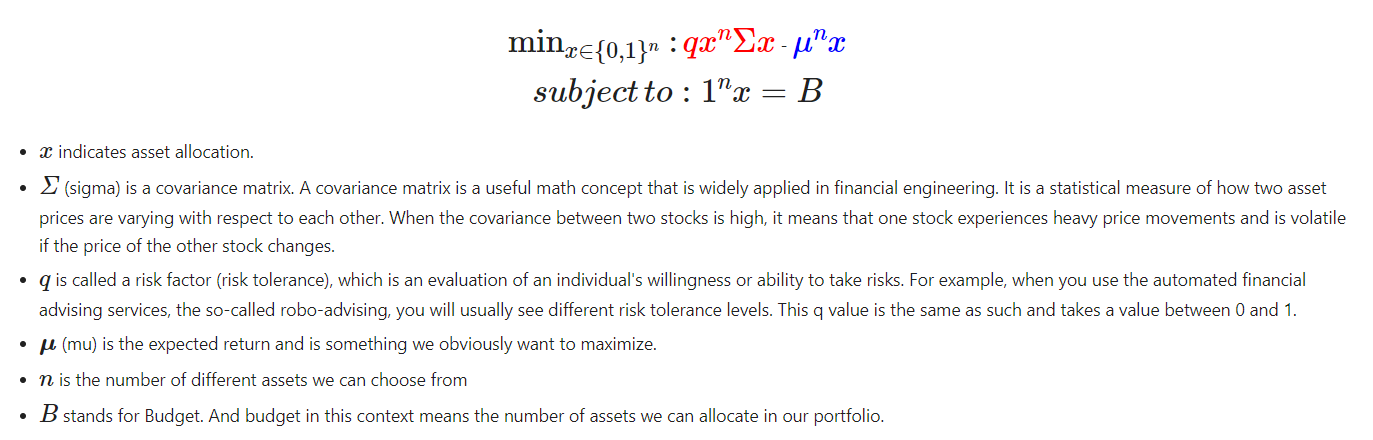
Where we are trying to optimize our portfolio distribution, or x, where the value (𝑥[𝑖]=1) indicates which stocks to pick and which not to pick (𝑥[𝑖]=0).

Stock Background

For the challenge we end up using historical stock data spanning between 1955-1985.

# Set parameters for assets and risk factor
num_assets = 4     # set number of assets to 4
q = 0.5                   # set risk factor to 0.5
budget = 2           # set budget as defined in the problem
seed = 132     #set random seed

# Generate time series data
stocks = [("STOCK%s" % i) for i in range(num_assets)]
data = RandomDataProvider(tickers=stocks,
                 start=datetime.datetime(1955,11,5),   
                 end=datetime.datetime(1985,10,26),  
                 seed=seed)
data.run()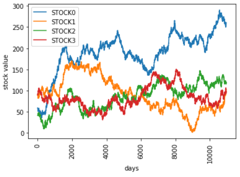

The next data point we want to gather is the historical expected return. This is simple to get based on our existing data.

mu = data.get_period_return_mean_vector()

print(mu)
---
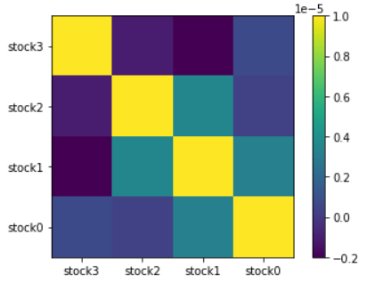
[1.59702144e-04 4.76518943e-04 2.39123234e-04 9.85029012e-05]

The last piece of information we need to is calculate the covariance between the stocks. Essentially we are calculating the relation of the stocks with the others.

• If two stocks increase and decrease simultaneously then the covariance value will be positive.
• If one increases while the other decreases then the covariance will be negative.

Modelling the Quadratic

The first part to optimizing our portfolio is to take the raw stock data we’ve established above and model it. Qiskit has a PortfolioOptimization class that can help do just that.

##############################
# Provide your code here

portfolio = PortfolioOptimization(expected_returns=mu, covariances=sigma, risk_factor=q, budget=budget)
qp = portfolio.to_quadratic_program()

##############################
print(qp)

And if we look at our qp object, we should notice a familiar quadratic structure we’ve encountered in previous challenges.

\ This file has been generated by DOcplex
\ ENCODING=ISO-8859-1
\Problem name: Portfolio optimization

Minimize
 obj: - 0.000159702144 x_0 - 0.000476518943 x_1 - 0.000239123234 x_2
      - 0.000098502901 x_3 + [ 0.000048831990 x_0^2 - 0.000002157372 x_0*x_1
      - 0.000004259230 x_0*x_2 + 0.000001413200 x_0*x_3 + 0.000997360142 x_1^2
      + 0.000007031887 x_1*x_2 + 0.000000737432 x_1*x_3 + 0.000287365468 x_2^2
      + 0.000006416382 x_2*x_3 + 0.000192316728 x_3^2 ]/2
Subject To
 c0: x_0 + x_1 + x_2 + x_3 = 2

Bounds
 0 <= x_0 <= 1
 0 <= x_1 <= 1
 0 <= x_2 <= 1
 0 <= x_3 <= 1

Binaries
 x_0 x_1 x_2 x_3
End

Excellent, I think we know where this headed now, so let’s go through and finish this off strong!

Classical Solution

As we normally do, let’s solve this classically so we have something to compare our quantum approaches.

exact_mes = NumPyMinimumEigensolver()
exact_eigensolver = MinimumEigenOptimizer(exact_mes)
result = exact_eigensolver.solve(qp)

print(result)
---
optimal function value: -0.00023285626449450194
optimal value: [1. 0. 1. 0.]
status: SUCCESS

VQE Solution

Now let’s go through a VQE solution. In this case the challenge provided us the optimizer already, so we just needed to create the parameterized circuit.

optimizer = SLSQP(maxiter=1000)  
algorithm_globals.random_seed = 1234
backend = Aer.get_backend('statevector_simulator')

##############################
# Provide your code here

ry = TwoLocal(num_assets, 'ry', 'cz', reps=3, entanglement='full')
quantum_instance = QuantumInstance(backend=backend, seed_simulator=seed, seed_transpiler=seed)
vqe = VQE(ry, optimizer=optimizer, quantum_instance=quantum_instance)

##############################

vqe_meo = MinimumEigenOptimizer(vqe)  #please do not change this code

result = vqe_meo.solve(qp)  #please do not change this code

print(result)    #please do not change this code
---
optimal function value: -0.00023285626449450194
optimal value: [1. 0. 1. 0.]
status: SUCCESS

And sure enough we see this matches our classical solution.

QAOA

Instead of duplicating the VQE solution for QAOA the challenge expanded the problem statement by allowing double the weight of individual stocks, and increasing our budget from 2 to 3.

q2 = 0.5     #Set risk factor to 0.5
budget2 = 3      #Set budget to 3

portfolio2 = PortfolioOptimization(expected_returns=mu, covariances=sigma, risk_factor=q2, budget=budget2, bounds=[[0,2],[0,2],[0,2],[0,2]])
qp2 = portfolio2.to_quadratic_program()

Now with the new portfolio quadratic function, we follow a similar approach and go through the QAOA solution.

optimizer = SLSQP(maxiter=1000)  
algorithm_globals.random_seed = 1234
backend = Aer.get_backend('statevector_simulator')

##############################
# Provide your code here 
quantum_instance = QuantumInstance(backend=backend, seed_simulator=seed, seed_transpiler=seed)
qaoa = QAOA(optimizer=optimizer, reps=3, quantum_instance=quantum_instance)

##############################

qaoa_meo = MinimumEigenOptimizer(qaoa) #please do not change this code

result2 = qaoa_meo.solve(qp2)  #please do not change this code

print(result2) #please do not change this code
---
optimal function value: -0.00032144003832501437
optimal value: [2. 0. 1. 0.]
status: SUCCESS

And just like that we’ve explored three separate ways to optimize our portfolio distribution, using real historical data.

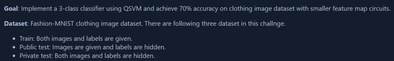
QSVM Image Classification

In this challenge we end up exploring Quantum Support Vector Machines (QSVM) to predict image classifications. Our goal is to expand on classical Machine Learning techniques and see not only how to translate them to a quantum approach, but improve upon the classical performance opening potential future applications.

**Goal** Implement a QSVM model for multiclass classification and predict labels accurately.

QSVM is a quantum version of the support vector machine (SVM), a classical machine learning algorithm. There are various approaches to QSVM, some aim to accelerate computation assuming fault-tolerant quantum computers, while others aim to achieve higher expressive power assuming noisy, near-term devices. In this challenge, we will focus on the latter.

Before we start solving the challenge we are presented with a breakdown on the various data encoding feature maps. The choice of which feature map we use will be influenced by the type of data we are working with understanding how these feature maps are structured will allow us to make a more educated choice.

Data Encoding with Feature Maps

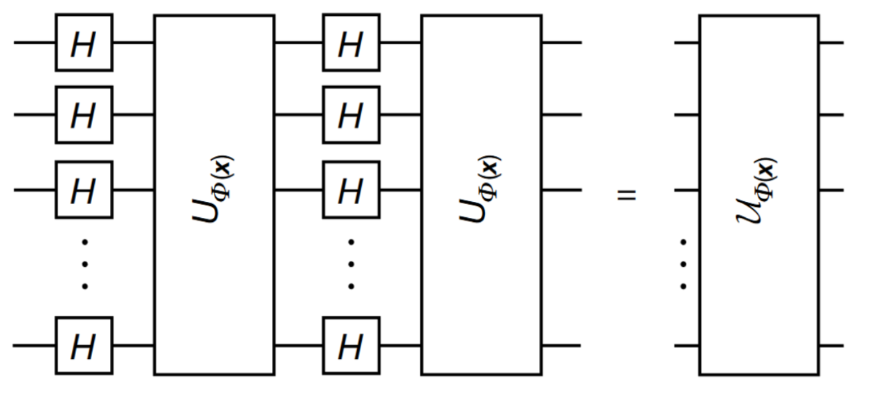
The first step we need to do to leverage a quantum implementation of a SVM is to bring our classical data into a quantum state. Basically we cannot just throw our classical data into a quantum circuit. We need to prepare the data in a way that will be usable with our circuits and techniques. We accomplish this by leveraging Feature Maps \(\phi(\mathbf{x})\) to bring the classical feature vector \(\mathbf{x}\) to the quantum state \(|\Phi(\mathbf{x})\rangle\langle\Phi(\mathbf{x})|\). This is facilitated by applying the unitary operation \(\mathcal{U}_{\Phi(\mathbf{x})}\) on the initial state \(|0\rangle^{n}\) where n is the number of features - the number of qubits being used for encoding.

PauliFeatureMap

The Pauli Feature Map contains layers of Hadamard gates interleaved with entangling blocks, \(U_{\Phi(\mathbf{x})}\), where within the entangling blocks, \(U_{\Phi(\mathbf{x})} : P_i \in \{ I, X, Y, Z \}\) denotes the Pauli matrices used to entangle the qubits and the index \(S\) describes connectivities between different qubits or datapoints: \(S \in \{\binom{n}{k}\ combinations,\ k = 1,... n \}\).

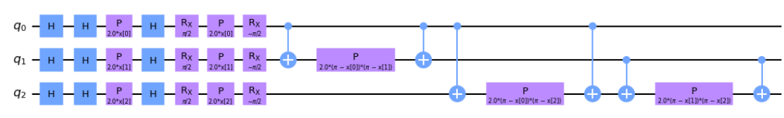
We can directly choose which pauli gates are used in our implementation if we have a direct need to customize the mapping.

# 3 features, depth 1
map_pauli = PauliFeatureMap(feature_dimension=3, reps=1, paulis = ['X', 'Y', 'ZZ'])
map_pauli.decompose().draw('mpl')

We define that there will be 3 features, represented as qubits, and a single repetition of the entanglement blocks.

ZFeatureMap

The ZFeatureMap is defined as \(k = 1, P_0 = Z\). Since the approach does not leverage any entanglement between the qubits this reduces the featuremap to being easily modelled classically, and as such would not present a quantum advantage in usage. It is however still a featuremap that can be represented quantumly, regardless of lack of advantage. Shown below is what the circuit looks like on implementation.

# 3 features, depth 2
map_z = ZFeatureMap(feature_dimension=3, reps=2)
map_z.decompose().draw('mpl')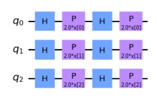

ZZFeatureMap

When \(k = 2, P_0 = Z, P_1 = ZZ\) this is called the ZZFeatureMap. In this approach we can also define the entanglement map and determine how the qubits are entangled amongst one another. In the first example you'll notice the qubits entangle in a linear cascade down the circuit, while the second shows a circular entanglement that cascades down and loops back to the start.

# 3 features, depth 1, linear entanglement
map_zz = ZZFeatureMap(feature_dimension=3, reps=1, entanglement='linear')
map_zz.decompose().draw('mpl')

# 3 features, depth 1, linear entanglement
map_zz = ZZFeatureMap(feature_dimension=3, reps=1, entanglement='circular')
map_zz.decompose().draw('mpl')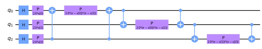

Parameterized Circuits

We can also create feature maps by using parameterized circuits of alternating rotation and entanglement layers. In both layers, parameterized circuit-blocks act on the circuit in a defined way. In the rotation layer, the blocks are applied stacked on top of each other, while in the entanglement layer according to the entanglement strategy. Each layer is repeated a number of times, and by default a final rotation layer is appended.

The main difference between NLocal and TwoLocal is that NLocal can have an arbitrary circuit block size, even smaller than the number of total qubits, while TwoLocal applies single qubit gates on all qubits and the entanglement uses two-qubit gates.

Let’s show the two implementing the same featuremap to illustrate the differences.

TwoLocal

twolocal = TwoLocal(num_qubits=3, reps=2, rotation_blocks=['ry','rz'], 
               entanglement_blocks='cx', entanglement='circular', insert_barriers=True)
twolocal.decompose().draw('mpl')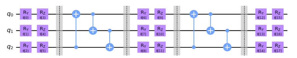

NLocal

twolocaln = NLocal(num_qubits=3, reps=2,
               rotation_blocks=[RYGate(Parameter('a')), RZGate(Parameter('a'))], 
               entanglement_blocks=CXGate(), 
               entanglement='circular', insert_barriers=True)
twolocaln.decompose().draw('mpl')

Quantum Kernel

With a better understanding of how to encode our data the next step is to understand how to determine the closeness between two sets of data. A quantum feature map, \(\phi(\mathbf{x})\), naturally gives rise to a quantum kernel, \(k(\mathbf{x}_i,\mathbf{x}_j)= \phi(\mathbf{x}_j)^\dagger\phi(\mathbf{x}_i)\), which can be seen as a measure of similarity: \(k(\mathbf{x}_i,\mathbf{x}_j)\) is large when \(\mathbf{x}_i\) and \(\mathbf{x}_j\) are close.

It might be clearer if we look at an example. First, let’s create our feature map and kernel. In this case since we have 5 features we are working with N_DIM will be 5, leading to 5 qubits in our featuremap.

pauli_map = PauliFeatureMap(feature_dimension=N_DIM, reps=1, paulis = ['X', 'Y', 'ZZ'])
pauli_kernel = QuantumKernel(feature_map=pauli_map, quantum_instance=Aer.get_backend('statevector_simulator'))

Now let’s look at our sample data, and compare the first and second sets that we will be working with.

print(f'First training data : {sample_train[0]}')
print(f'Second training data: {sample_train[1]}')
---
First training data : [-0.4755618  -0.42255659  0.30043225  0.00532007 -0.89492354]
Second training data: [ 0.05258865 -0.6720529  -0.28177088  0.02276329 -0.38711636]

Putting them both together, let’s embed our sample data into the featuremap we selected.

pauli_circuit = pauli_kernel.construct_circuit(sample_train[0], sample_train[1])
pauli_circuit.decompose().decompose().draw(output='mpl')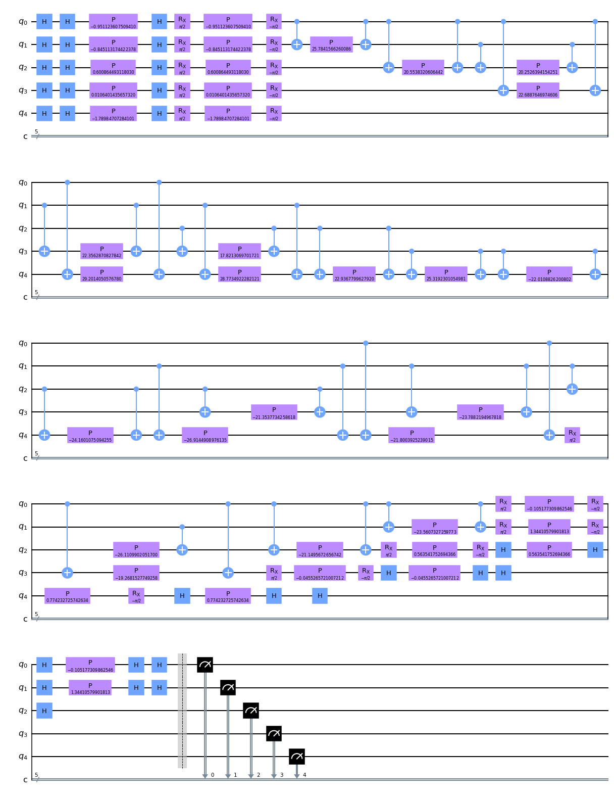

We then simulate the circuit and calculate the transition amplitude for the two data sets.

backend = Aer.get_backend('qasm_simulator')
job = execute(pauli_circuit, backend, shots=8192, 
              seed_simulator=1024, seed_transpiler=1024)
counts = job.result().get_counts(pauli_circuit)

print(f"Transition amplitude: {counts['0'*N_DIM]/sum(counts.values())}")
---
Transition amplitude: 0.028564453125

What would happen if we changed the two data sets we are using? If we used the same data set in a perfect 1-to-1 matching, how would that change the transition amplitude? I leave it to you all to repeat the experiment above and find out!

QSVM for 3-class classification

Everything we’ve looked at so far has prepared us for the challenge component. With the techniques explored we are presented with the actual challenge statement.

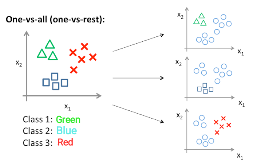
In my solution I approached with the one-vs-rest approach. What this ultimately means is that knowing the data set had three possible breakdowns I will need to implement three different classifiers together, then combine the output to hopefully come out with the right label.

One-vs-Rest: In this approach, multi-class classification is achieved by combining classifiers for each class that classifies the class as positive and the others as negative. Since one classifier is required for each class, the total number of classifiers required for N-class classification is N. The advantage is that fewer classifiers are needed, and the disadvantage is that the labels are likely to be imbalanced in each classification.

The approach we will be taking is loosely broken down to the following steps:

• Load the data
• Preprocess the data
  • Standardization
  • Principal component analysis (PCA)
  • Normalization
• Run through label 0 classification
• Run through label 2 classification
• Run through label 3 classification
• For test data determine which label had the highest percentage chance

And putting it all together we get the following solution.

# Load MNIST dataset
DATA_PATH = './resources/ch3_part2.npz'
data = np.load(DATA_PATH)

sample_train = data['sample_train']
labels_train = data['labels_train']
sample_test = data['sample_test']

# Split train data
sample_train, sample_val, labels_train, labels_val = train_test_split(
    sample_train, labels_train, test_size=0.2, random_state=42)

# Standardize
standard_scaler = StandardScaler()
sample_train = standard_scaler.fit_transform(sample_train)
sample_val = standard_scaler.transform(sample_val)
sample_test = standard_scaler.transform(sample_test)

# Reduce dimensions
N_DIM = 5
pca = PCA(n_components=N_DIM)
sample_train = pca.fit_transform(sample_train)
sample_val = pca.transform(sample_val)
sample_test = pca.transform(sample_test)

# Normalize
min_max_scaler = MinMaxScaler((-1, 1))
sample_train = min_max_scaler.fit_transform(sample_train)
sample_val = min_max_scaler.transform(sample_val)
sample_test = min_max_scaler.transform(sample_test)

# 0 vs. rest
labels_train_0 = np.where(labels_train==0, 1, 0)
labels_val_0 = np.where(labels_val==0, 1, 0)
pauli_map_0 = ZZFeatureMap(feature_dimension=N_DIM, reps=1, entanglement='linear')
kernel_0 = QuantumKernel(feature_map=pauli_map_0, quantum_instance=Aer.get_backend('statevector_simulator'))
svc_0 = SVC(kernel='precomputed', probability=True)
matrix_train_0 = kernel_0.evaluate(x_vec=sample_train)
svc_0.fit(matrix_train_0, labels_train_0)
matrix_val_0 = kernel_0.evaluate(x_vec=sample_val, y_vec=sample_train)
pauli_score_0 = svc_0.score(matrix_val_0, labels_val_0)
print(f'Accuracy of discriminating between label 0 and others: {pauli_score_0*100}%')
matrix_test_0 = kernel_0.evaluate(x_vec=sample_test, y_vec=sample_train)
pred_0 = svc_0.predict_proba(matrix_test_0)[:, 1]
print(f'Probability of label 0: {np.round(pred_0, 2)}')

# 2 vs. rest
labels_train_2 = np.where(labels_train==2, 1, 0)
labels_val_2 = np.where(labels_val==2, 1, 0)
pauli_map_2 = ZZFeatureMap(feature_dimension=N_DIM, reps=1, entanglement='linear')
kernel_2 = QuantumKernel(feature_map=pauli_map_2, quantum_instance=Aer.get_backend('statevector_simulator'))
svc_2 = SVC(kernel='precomputed', probability=True)
matrix_train_2 = kernel_2.evaluate(x_vec=sample_train)
svc_2.fit(matrix_train_2, labels_train_2)
matrix_val_2 = kernel_2.evaluate(x_vec=sample_val, y_vec=sample_train)
pauli_score_2 = svc_2.score(matrix_val_2, labels_val_2)
print(f'Accuracy of discriminating between label 2 and others: {pauli_score_2*100}%')
matrix_test_2 = kernel_2.evaluate(x_vec=sample_test, y_vec=sample_train)
pred_2 = svc_2.predict_proba(matrix_test_2)[:, 1]
print(f'Probability of label 2: {np.round(pred_2, 2)}')

# 3 vs. rest
labels_train_3 = np.where(labels_train==3, 1, 0)
labels_val_3 = np.where(labels_val==3, 1, 0)
pauli_map_3 = ZZFeatureMap(feature_dimension=N_DIM, reps=1, entanglement='linear') 
kernel_3 = QuantumKernel(feature_map=pauli_map_3, quantum_instance=Aer.get_backend('statevector_simulator'))
svc_3 = SVC(kernel='precomputed', probability=True)
matrix_train_3 = kernel_3.evaluate(x_vec=sample_train)
svc_3.fit(matrix_train_3, labels_train_3)
matrix_val_3 = kernel_3.evaluate(x_vec=sample_val, y_vec=sample_train)
pauli_score_3 = svc_3.score(matrix_val_3, labels_val_3)
print(f'Accuracy of discriminating between label 3 and others: {pauli_score_3*100}%')
matrix_test_3 = kernel_3.evaluate(x_vec=sample_test, y_vec=sample_train)
pred_3 = svc_3.predict_proba(matrix_test_3)[:, 1]
print(f'Probability of label 3: {np.round(pred_3, 2)}')

pred_test = []

i=0
while i < pred_0.size:
    if pred_0[i] > pred_2[i] and pred_0[i] > pred_3[i]:
        print (f'{np.round(pred_0[i], 2)} , {np.round(pred_2[i], 2)} , {np.round(pred_3[i], 2)}  = 0')
        pred_test.append(0)
    if pred_2[i] > pred_0[i] and pred_2[i] > pred_3[i]:
        print (f'{np.round(pred_0[i], 2)} , {np.round(pred_2[i], 2)} , {np.round(pred_3[i], 2)}  = 2')
        pred_test.append(2)
    if pred_3[i] > pred_2[i] and pred_3[i] > pred_0[i]:
        print (f'{np.round(pred_0[i], 2)} , {np.round(pred_2[i], 2)} , {np.round(pred_3[i], 2)}  = 3')
        pred_test.append(3)
    i=i+1

print(pred_test)
pred_test = np.array(pred_test)
print(pred_test)
##############################

grade_ex3c(pred_test, sample_train, 
           standard_scaler, pca, min_max_scaler,
           kernel_0, kernel_2, kernel_3,
           svc_0, svc_2, svc_3)

I added quite a few print statements and breaks throughout the testing process to see if my adjustments were making any differences. By the end I was able to quickly visualize what each testing data entry would look like from a probability perspective and how that influenced the final selection. After a series of adjustments to the featuremap I was able to get well above the 70% threshold requirement on the training data and was thankfully rewarded with a successful submission to the grader.

Accuracy of discriminating between label 0 and others: 95.0%
Probability of label 0: [0.97 0.96 0.07 0.19 0.11 0.08 0.96 0.51 0.97 0.94 0.09 0.47 0.05 0.38
 0.1 0.06 0.12 0.85 0.1  0.22]

Accuracy of discriminating between label 2 and others: 85.0%
Probability of label 2: [0.05 0.06 0.04 0.18 0.18 0.19 0.07 0.44 0.05 0.07 0.1 0.42 0.94 0.6
 0.12 0.96 0.09 0.06 0.24 0.55]

Accuracy of discriminating between label 3 and others: 95.0%
Probability of label 3: [0.07 0.07 0.91 0.57 0.65 0.71 0.04 0.05 0.07 0.06 0.82 0.07 0.08 0.09
 0.84 0.06 0.81 0.13 0.71 0.09]

0.97 , 0.05 , 0.07  = 0
0.96 , 0.06 , 0.07  = 0
0.07 , 0.04 , 0.91  = 3
0.19 , 0.18 , 0.57  = 3
0.11 , 0.18 , 0.65  = 3
0.08 , 0.19 , 0.71  = 3
0.96 , 0.07 , 0.04  = 0
0.51 , 0.44 , 0.05  = 0
0.97 , 0.05 , 0.07  = 0
0.94 , 0.07 , 0.06  = 0
0.09 , 0.1 , 0.82  = 3
0.47 , 0.42 , 0.07  = 0
0.05 , 0.94 , 0.08  = 2
0.38 , 0.6 , 0.09  = 2
0.1 , 0.12 , 0.84  = 3
0.06 , 0.96 , 0.06  = 2
0.12 , 0.09 , 0.81  = 3
0.85 , 0.06 , 0.13  = 0
0.1 , 0.24 , 0.71  = 3
0.22 , 0.55 , 0.09  = 2
[0, 0, 3, 3, 3, 3, 0, 0, 0, 0, 3, 0, 2, 2, 3, 2, 3, 0, 3, 2]
[0 0 3 3 3 3 0 0 0 0 3 0 2 2 3 2 3 0 3 2]

Submitting your answer for 3c. Please wait...
Congratulations 🎉! Your answer is correct and has been submitted.
Your score is 282.

Conclusion

My experience with previous IBM Qiskit events has been positive and this event was no exception. I mentioned at the start of this article that this event felt like a personal pivotal point in my quantum journey. I went from reading theoretical approaches of quantum computing back in the mid 2000s, to applying those conceptual theories in code as of 2019. Now with this event just a few short years later I feel that next step of solving something practical is much, much closer. The two challenges of the event I covered were, while still arguably toy examples, still using real data publicly available. It would not be a stretch to expand either of the challenges to either include more stocks and boundaries, or a larger pool of potential classifications.

As the engineering challenge of designing and creating reliable Quantum hardware continues to make progress, we are moving closer and closer to a time where we are able to integrate quantum computing to our daily lives. The time is now to start learning how this integration can take place and be ready for when it is possible.

Excited to participate in the next event and see where this journey continues!

Thanks folks, until next time!