
Introduction
![]()
The IBM Quantum Challenge Fall 2022 runs from 9:00 a.m. US Eastern on Friday, November 11 until 9:00 a.m. US Eastern on Friday, November 18, and will focus on two trailblazing offerings unveiled by IBM Quantum in recent years: Qiskit Runtime and Primitives. Participants in this year’s Fall Challenge will enjoy eight days of learning, exploring the most promising applications in quantum computing through special missions distributed across four levels of ascending difficulty
Qiskit’s Fall 2022 event focused on two new offerings:
Primitives - foundational, elementary, building blocks for users to perform quantum computations, developers to implement quantum algorithms, and researchers to solve complex problems and deliver new applications.
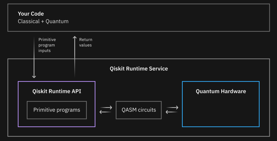
Runtime - the Qiskit Runtime service has been built on the concept of containerized execution; an execution model, where you have multiple elements of computation packaged and run portably on any system.
In what has turned out to be one of the best narratives during these Quantum events, the Qiskit Fall 2022 event put us in the captain’s seat of the Earth’s first faster-than-light starship solving quantum-inspired problems in an attempt to keep the crew safe along the mission. This was my first experience with Qiskit’s Primitives and Runtime execution and I can see the benefit of using this type of workload management, especially when experimenting with many iterations of small variations.
Without any further ado, let’s jump into the challenges.
Lab1 - Qiskit Runtime and Primitives

Bernstein Vazirani
The first lab is all about learning the fundamentals of Primitives and how to practically use them. Before we jump right into that however, we are presented with the background of the Bernstein Vazirani function. The Bernstein Vazirani function is a fundamental quantum algorithm which showed that there can be advantages in using a quantum computer as a computational tool for more complex problems.
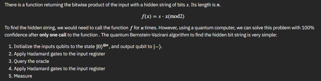
Having been stepped through a concrete example, our first challenge was to define a BV function that could work for any “hidden string”.
def bernstein_vazirani(string):

    # Save the length of string
    string_length = len(string)

    # Make a quantum circuit
    qc = QuantumCircuit(string_length+1, string_length)

    # Initialize each input qubit to apply a Hadamard gate and output qubit to |->
    qc.h(string_length)
    qc.z(string_length)

    for i in range(string_length):
        qc.h(i)

    # Apply an oracle for the given string
    # Note: In Qiskit, numbers are assigned to the bits in a string from right to left
    string = string[::-1] # reverse s to fit qiskit's qubit ordering
    for q in range(string_length):
        if string[q] == '0':
            qc.i(q)
        else:
            qc.cx(q, string_length)

    # Apply Hadamard gates after querying the oracle
    for i in range(string_length):
        qc.h(i)

    # Measurement
    qc.measure(range(string_length), range(string_length))

return qc 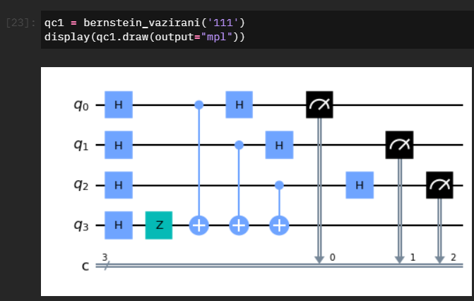
Sampler & Parameterized Circuits
The next concept we are introduced to is parameterized circuit - which in this case allows us to dynamically bind P-gate rotations to the sample circuit. We combine this with an introduction to using Sampler and passing our circuit through Runtime.
theta = Parameter('theta')

qc = QuantumCircuit(2,1)
qc.x(1)
qc.h(0)
qc.cp(theta,0,1)
qc.h(0)
qc.measure(0,0)

qc.draw()

options = Options(simulator={"seed_simulator": 42}, resilience_level=0) # Do not change values in simulator
circuits = [qc.bind_parameters({theta: theta_val}) for [theta_val] in individual_phases]

with Session(service=service, backend=backend):
    sampler = Sampler(options=options)
    job = sampler.run(circuits=circuits)
    result = job.result()

from qc_grader.challenges.fall_2022 import grade_lab1_ex2
grade_lab1_ex2(result) # Expected result type: SamplerResult
Estimator
With the basics covered, we jump into a multi-step exercise to explore how we can pass multiple sets of parameters and circuits to Estimator and execute it once to gather the expectation values.

# Make three random circuits using RealAmplitudes
psi1 = RealAmplitudes(5, reps=2)
psi2 = RealAmplitudes(5, reps=3)
psi3 = RealAmplitudes(5, reps=4)

# Make hamiltonians using SparsePauliOp
H1 = SparsePauliOp.from_list([("IIZXI", 1), ("YIIIY", 3)])
H2 = SparsePauliOp.from_list([("IXIII", 2)])
H3 = SparsePauliOp.from_list([("IIYII", 3), ("IXIZI", 5)])

# Make a random list for theta between 0 and 1
theta1 = np.linspace(0, 1, 15)
theta2 = np.linspace(0, 1, 20)
theta3 = np.linspace(0, 1, 25)

# Use the Estimator to calculate each expectation value

with Session(service=service, backend=backend):
    options = Options(simulator={"seed_simulator": 42}, resilience_level=0) # Do not change values in simulator

    estimator = Estimator(options=options)
    job = estimator.run(circuits=[psi1,psi2,psi3],parameter_values=[theta1,theta2,theta3],observables=[H1,H2,H3])
result = job.result() 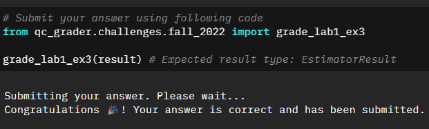
Quantum Error Mitigation & Suppression
The last part of the first lab was to explore error mitigation and suppression in context of Qiskit Runtime.
Sampler & M3
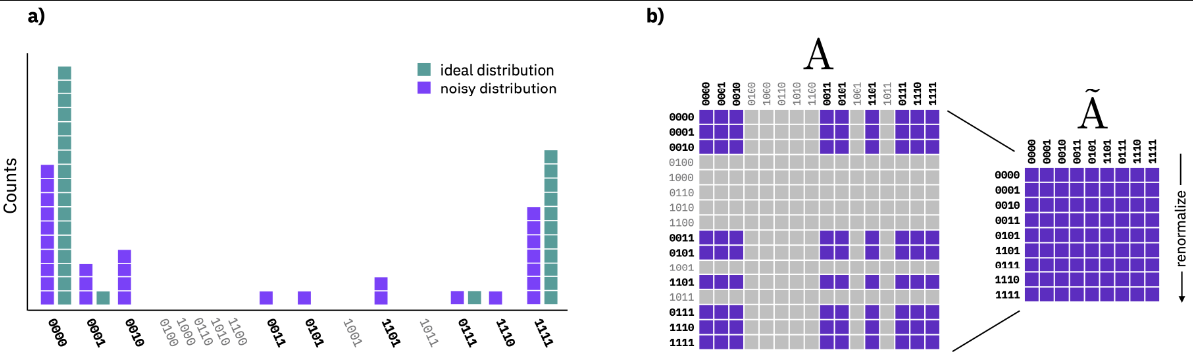
Qiskit Sampler allows us to leverage M3 (Matrix-free measurement mitigation) error mitigation routines. As part of the lab we are given a quick background into noise and M3.
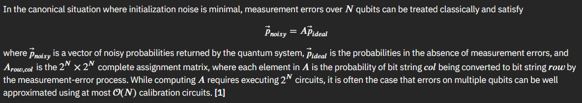
M3 works in a reduced subspace that is defined by the noisy input that need to be corrected. Since the input can be smaller than the full dimensionality of Hilbert space, the resulting linear system of equations is much easier to solve.
$$(\overset{\sim}{A})^{-1}\overset{\sim}{A}\vec{p}_{ideal} = (\overset{\sim}{A})^{-1}\vec{p}_{noisy} $$
All that is left is putting the M3 approach to code and testing it out.
from qiskit.providers.fake_provider import FakeManila
from qiskit_aer.noise import NoiseModel

# Import FakeBackend
fake_backend = FakeManila()
noise_model = NoiseModel.from_backend(fake_backend)

# Set options to include noise_model
options = Options(simulator={
    "noise_model": noise_model,
    "seed_simulator": 42,
}, resilience_level=0)

# Set options to include noise_model and resilience_level
options_with_em = Options(
    simulator={
        "noise_model": noise_model,
        "seed_simulator": 42,
    },
    resilience_level=1
)

with Session(service=service, backend=backend):
    sampler = Sampler(options=options)
    job = sampler.run(circuits=[qc]*len(phases), parameter_values=individual_phases)
    param_results = job.result()
    prob_values = [1-dist[0] for dist in param_results.quasi_dists]

    sampler = Sampler(options=options_with_em)
    job = sampler.run(circuits=[qc]*len(phases), parameter_values=individual_phases)
    param_results = job.result()
prob_values_with_em = [1-dist[0] for dist in param_results.quasi_dists] 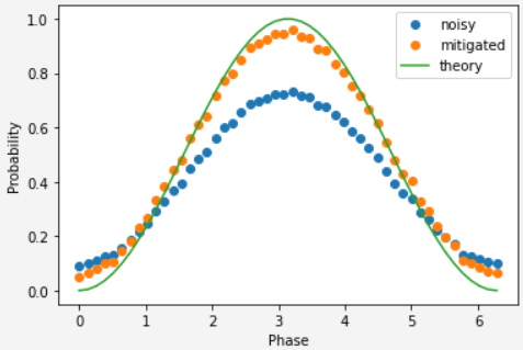
Estimator & ZNE
We were then introduced to Zero-Noise Extrapolation error mitigation and explored how to implement it using Qiskit Estimators.
With ZNE a quantum program is altered to run at different effect levels of processor noise. The result of the computation is extrapolated to an estimated value at a noiseless level. There several methods for estimating the value:

Of which Qiskit implements the digital approach.
# Set options to activate T-Rex Error Mitigation module
options_with_em = Options(
    simulator={
        "noise_model": noise_model,
        "seed_simulator": 42,
    },
    resilience_level=1 # You may change the value here. resilience_level = 1 will activate TREX
)
with Session(service=service, backend=backend):
    estimator = Estimator(options=options)
    job = estimator.run(circuits=[qc_no_meas]*len(phases), parameter_values=individual_phases, observables=[ZZ]*len(phases))
    param_results = job.result()
    exp_values = param_results.values

    estimator = Estimator(options=options_with_em)
    job = estimator.run(circuits=[qc_no_meas]*len(phases), parameter_values=individual_phases, observables=[ZZ]*len(phases))
    param_results = job.result()
exp_values_with_em = param_results.values 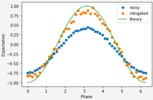
Lab2 - Quantum Machine Learning
The focus of the second lab is to implement the previously learned M3 error mitigation to various machine learning applications. Before we jump straight into error mitigation however the notebook goes over the basics of quantum machine learning, specifically data embedding and ansatz.
In quantum machine learning, a quantum feature map transforms $\vec{x} \rightarrow | \phi(\vec{x})\rangle$ using a unitary transformation $\vec{U_\phi}(\vec{x})$, which is typically a parameterized quantum circuit. Parametrized quantum circuits in quantum machine learning tend to be used for encoding data and as a quantum model. Their parameters are determined by the data being encoded and optimization process. They can generate a key subset of the states within the output Hilbert space and it allows them to be used as machine learning model
Throughout this notebook we will be using a RealAmplitudes 2-local ansatz:
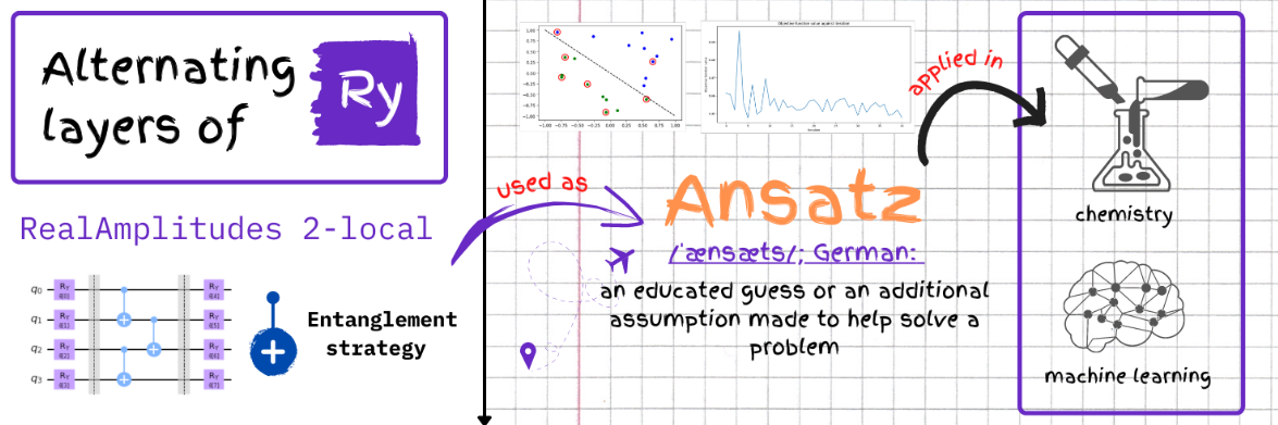
At which point we are given a sample data which we need to embed in a quantum circuit we define.
from qiskit.circuit.library import RealAmplitudes

def lab2_ex1():
    # build your code here
    qc = QuantumCircuit(4)
    qc = RealAmplitudes(4, entanglement='pairwise',reps=1)
    #
    return qc


qc = lab2_ex1()
encode = qc.bind_parameters(sample_train[0])
encode.measure_all()
encode.decompose().draw("mpl") 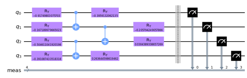
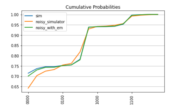
We then ran our circuit on an ideal and noisy simulator to see the effects of the noise on our output. We will be using this as a base measurement, and then work on incorporating error mitigation to see the overall impact.
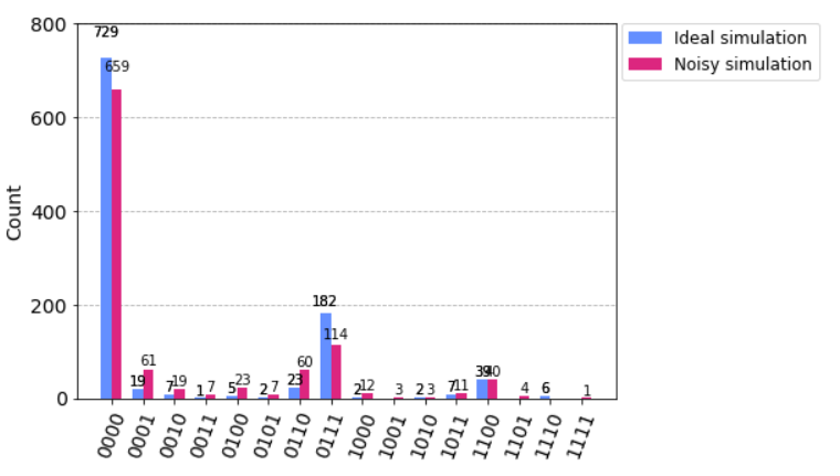
Adding in the M3 mitigation similarly to the first notebook:
# Do not change the seed of simulatior in Options
options = Options(simulator={"seed_simulator": 1234},resilience_level=0)
shots = 10000
with Session(service=service, backend=backend):
    sampler = Sampler(options=options)
    job = sampler.run(circuits=[qc], parameter_values=[sample_train[0]], shots=shots)
    samples_sim = job.result()
Once we run this mitigated approach on the noisy backend we can then compare the approaches and see the accuracy differences between them all:
Where fidelity is the closeness of two quantum states. Given two states $|\psi\rangle = U|0\rangle$ and $|\varphi\rangle = V|0\rangle$ generated by the unitaries $U$ and $V$, the fidelity is defined as
\[\left|\langle \psi \mid \varphi \rangle\right|^2 = \left|\langle 0 \mid U^{\dagger} V \mid 0\rangle \right|^2\]And this can be implemented in code by the following circuit:
# parametrized circuit defining U first state
circuit_1 = RealAmplitudes(4, reps=1, entanglement='pairwise',
                           insert_barriers=True, parameter_prefix='x')

# parametrized circuit V defining second state
circuit_2 = RealAmplitudes(4, reps=1, entanglement='pairwise',
                           insert_barriers=True, parameter_prefix='y')

# combining circuits to evaluate U^dagger V
fidelity_circuit = circuit_1.copy()
fidelity_circuit.append(circuit_2.inverse().decompose(), range(fidelity_circuit.num_qubits))
fidelity_circuit.measure_all()

# drawing resulting circuit to estimate fidelity
fidelity_circuit.decompose().draw('mpl') 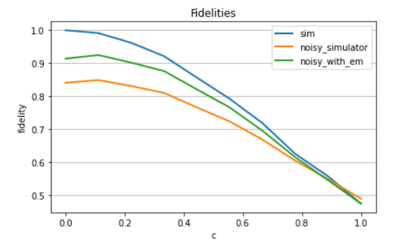
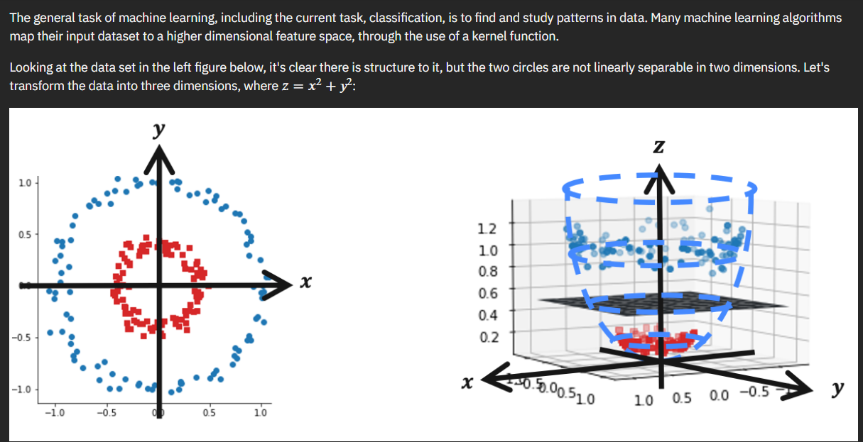
Quantum Kernels & QSVMs
Now that we have a way to implement error correction, and a way to calculate the resulting fidelity, we can explore quantum kernels.
Machine learning algorithms can map the input dataset to higher dimensional feature map using kernel function, $k(\vec{x}_i, \vec{x}_j) = \langle f(\vec{x}_i), f(\vec{x}_j) \rangle $ where $k$ is kernel function, $\vec{x}_i, \vec{x}_j$ are $n$ dimensional inputs, $f$ is map from $n$-dimension to $m$-dimension space. When we consider that data is finite, the quantum kernel can be expressed as matrix
\[K_{ij}=|\langle\phi^{\dagger}(\vec{x}_j)|\phi(\vec{x}_i)\rangle|^2\]and since we can express the quantum kernel as a parameterized circuit with \(n\) qubits that becomes:
\[|\langle\phi^{\dagger}(\vec{x}_j)|\phi(\vec{x}_i)\rangle|^2 = |\langle 0^{\otimes n}|U^{\dagger}_{\phi(\vec{x}_j)} U_{\phi(\vec{x}_i)}|0^{\otimes n} \rangle |^2\] 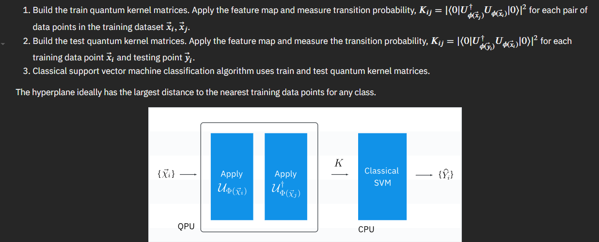
The code to implement this is simplistic with leveraging Sampler similarly to how we have done up to now.
with Session(service=service, backend=backend):
    sampler = Sampler(options=options_with_em)# build your code here
    job =  sampler.run(circuits=[fidelity_circuit]*300, parameter_values=data_append(n,sample_train,sample_train), shots=10000) # build your code here
    quantum_kernel_em = job.result()

kernel_em = []
for i in range(circuit_num):
    kernel_em += [quantum_kernel_em.quasi_dists[i][0]]

K = np.zeros((n, n))
count = 0
for i in range(n):
    for j in range(n):
        if j<i:
            K[i,j] = K[j,i]
        else:
            if j==i:
                K[i,j] = 1
            else:
                K[i,j] = kernel_em[count]
                count+=1
plot_matrix(K, 'kernel matrix (em)') 
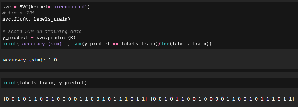
And lastly we can check the accuracy of our training:
Lab3 - Quantum Optimization
The third notebook will be building on the first two and explore optimization in the case of a Traveling Salesman Problem.
After being given a quick explanation of what a TSP problem is, the first part of our challenge is to model the situation into a graph format.
n = 4
num_qubits =  n**2

#### enter your code above ####

tsp = Tsp.create_random_instance(n, seed=123)
adj_matrix = nx.to_numpy_matrix(tsp.graph)
print("distance\n", adj_matrix)

colors = ["r" for node in tsp.graph.nodes]
pos = [tsp.graph.nodes[node]["pos"] for node in tsp.graph.nodes]
draw_graph(tsp.graph, colors, pos)

distance
 [[ 0. 48. 91. 33.]
 [48.  0. 63. 71.]
 [91. 63.  0. 92.]
[33. 71. 92. 0.]] 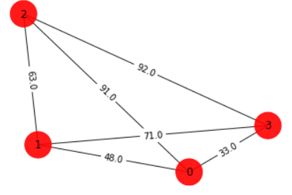
Skipping the code as we are more interested in the quantum approach, however we go through this example classically to have a working shortest path to compare in our quantum application.
Quadratic Representation
To approach solving this problem quantumly, we first start with modeling our graph as a quadratic.
qp = tsp.to_quadratic_program()
print(qp.prettyprint())

Problem name: TSP

Minimize
  48*x_0_0*x_1_1 + 48*x_0_0*x_1_3 + 91*x_0_0*x_2_1 + 91*x_0_0*x_2_3
  + 33*x_0_0*x_3_1 + 33*x_0_0*x_3_3 + 48*x_0_1*x_1_0 + 48*x_0_1*x_1_2
  + 91*x_0_1*x_2_0 + 91*x_0_1*x_2_2 + 33*x_0_1*x_3_0 + 33*x_0_1*x_3_2
  + 48*x_0_2*x_1_1 + 48*x_0_2*x_1_3 + 91*x_0_2*x_2_1 + 91*x_0_2*x_2_3
  + 33*x_0_2*x_3_1 + 33*x_0_2*x_3_3 + 48*x_0_3*x_1_0 + 48*x_0_3*x_1_2
  + 91*x_0_3*x_2_0 + 91*x_0_3*x_2_2 + 33*x_0_3*x_3_0 + 33*x_0_3*x_3_2
  + 63*x_1_0*x_2_1 + 63*x_1_0*x_2_3 + 71*x_1_0*x_3_1 + 71*x_1_0*x_3_3
  + 63*x_1_1*x_2_0 + 63*x_1_1*x_2_2 + 71*x_1_1*x_3_0 + 71*x_1_1*x_3_2
  + 63*x_1_2*x_2_1 + 63*x_1_2*x_2_3 + 71*x_1_2*x_3_1 + 71*x_1_2*x_3_3
  + 63*x_1_3*x_2_0 + 63*x_1_3*x_2_2 + 71*x_1_3*x_3_0 + 71*x_1_3*x_3_2
  + 92*x_2_0*x_3_1 + 92*x_2_0*x_3_3 + 92*x_2_1*x_3_0 + 92*x_2_1*x_3_2
  + 92*x_2_2*x_3_1 + 92*x_2_2*x_3_3 + 92*x_2_3*x_3_0 + 92*x_2_3*x_3_2

Subject to
  Linear constraints (8)
    x_0_0 + x_0_1 + x_0_2 + x_0_3 == 1  'c0'
    x_1_0 + x_1_1 + x_1_2 + x_1_3 == 1  'c1'
    x_2_0 + x_2_1 + x_2_2 + x_2_3 == 1  'c2'
    x_3_0 + x_3_1 + x_3_2 + x_3_3 == 1  'c3'
    x_0_0 + x_1_0 + x_2_0 + x_3_0 == 1  'c4'
    x_0_1 + x_1_1 + x_2_1 + x_3_1 == 1  'c5'
    x_0_2 + x_1_2 + x_2_2 + x_3_2 == 1  'c6'
    x_0_3 + x_1_3 + x_2_3 + x_3_3 == 1  'c7'

  Binary variables (16)
    x_0_0 x_0_1 x_0_2 x_0_3 x_1_0 x_1_1 x_1_2 x_1_3 x_2_0 x_2_1 x_2_2 x_2_3
    x_3_0 x_3_1 x_3_2 x_3_3
This is not all that is required however. We also need to convert this quadratic into a form that can be used in a quantum circuit. Enter the Ising Hamiltonian. An Ising Hamiltonian is a representation of the energy in a particular system. This allows us to use eigensolvers to find the minimum energy, which represents the shortest path solution of our original graph problem.
We can get the Ising representation of our quadratic using built in functions of Qiskit.
from qiskit_optimization.converters import QuadraticProgramToQubo

#### enter your code below ####

qp2qubo = QuadraticProgramToQubo()   #instatiate qp to qubo class
qubo = qp2qubo.convert(qp)      # convert quadratic program to qubo
qubitOp, offset = qubo.to_ising()    #convert qubo to ising

#### enter your code above ####

print("Offset:", offset)
print("Ising Hamiltonian:", str(qubitOp))

Offset: 51756.0
Ising Hamiltonian: -6456.0 * IIIIIIIIIIIIIIIZ
- 6456.0 * IIIIIIIIIIIIIIZI
- 6456.0 * IIIIIIIIIIIIIZII
- 6456.0 * IIIIIIIIIIIIZIII
- 6461.0 * IIIIIIIIIIIZIIII
- 6461.0 * IIIIIIIIIIZIIIII
- 6461.0 * IIIIIIIIIZIIIIII
- 6461.0 * IIIIIIIIZIIIIIII
- 6493.0 * IIIIIIIZIIIIIIII
- 6493.0 * IIIIIIZIIIIIIIII
- 6493.0 * IIIIIZIIIIIIIIII
- 6493.0 * IIIIZIIIIIIIIIII
- 6468.0 * IIIZIIIIIIIIIIII
- 6468.0 * IIZIIIIIIIIIIIII
- 6468.0 * IZIIIIIIIIIIIIII
- 6468.0 * ZIIIIIIIIIIIIIII
+ 1592.5 * IIIIIIIIIIIIIIZZ
+ 1592.5 * IIIIIIIIIIIIIZIZ
+ 1592.5 * IIIIIIIIIIIIIZZI
+ 1592.5 * IIIIIIIIIIIIZIIZ
+ 1592.5 * IIIIIIIIIIIIZIZI
+ 1592.5 * IIIIIIIIIIIIZZII
+ 1592.5 * IIIIIIIIIIIZIIIZ
+ 12.0 * IIIIIIIIIIIZIIZI
+ 12.0 * IIIIIIIIIIIZZIII
+ 12.0 * IIIIIIIIIIZIIIIZ
+ 1592.5 * IIIIIIIIIIZIIIZI
+ 12.0 * IIIIIIIIIIZIIZII
+ 1592.5 * IIIIIIIIIIZZIIII
+ 12.0 * IIIIIIIIIZIIIIZI
+ 1592.5 * IIIIIIIIIZIIIZII
+ 12.0 * IIIIIIIIIZIIZIII
+ 1592.5 * IIIIIIIIIZIZIIII
+ 1592.5 * IIIIIIIIIZZIIIII
+ 12.0 * IIIIIIIIZIIIIIIZ
+ 12.0 * IIIIIIIIZIIIIZII
+ 1592.5 * IIIIIIIIZIIIZIII
+ 1592.5 * IIIIIIIIZIIZIIII
+ 1592.5 * IIIIIIIIZIZIIIII
+ 1592.5 * IIIIIIIIZZIIIIII
+ 1592.5 * IIIIIIIZIIIIIIIZ
+ 22.75 * IIIIIIIZIIIIIIZI
+ 22.75 * IIIIIIIZIIIIZIII
+ 1592.5 * IIIIIIIZIIIZIIII
+ 15.75 * IIIIIIIZIIZIIIII
+ 15.75 * IIIIIIIZZIIIIIII
+ 22.75 * IIIIIIZIIIIIIIIZ
+ 1592.5 * IIIIIIZIIIIIIIZI
+ 22.75 * IIIIIIZIIIIIIZII
+ 15.75 * IIIIIIZIIIIZIIII
+ 1592.5 * IIIIIIZIIIZIIIII
+ 15.75 * IIIIIIZIIZIIIIII
+ 1592.5 * IIIIIIZZIIIIIIII
+ 22.75 * IIIIIZIIIIIIIIZI
+ 1592.5 * IIIIIZIIIIIIIZII
+ 22.75 * IIIIIZIIIIIIZIII
+ 15.75 * IIIIIZIIIIZIIIII
+ 1592.5 * IIIIIZIIIZIIIIII
+ 15.75 * IIIIIZIIZIIIIIII
+ 1592.5 * IIIIIZIZIIIIIIII
+ 1592.5 * IIIIIZZIIIIIIIII
+ 22.75 * IIIIZIIIIIIIIIIZ
+ 22.75 * IIIIZIIIIIIIIZII
+ 1592.5 * IIIIZIIIIIIIZIII
+ 15.75 * IIIIZIIIIIIZIIII
+ 15.75 * IIIIZIIIIZIIIIII
+ 1592.5 * IIIIZIIIZIIIIIII
+ 1592.5 * IIIIZIIZIIIIIIII
+ 1592.5 * IIIIZIZIIIIIIIII
+ 1592.5 * IIIIZZIIIIIIIIII
+ 1592.5 * IIIZIIIIIIIIIIIZ
+ 8.25 * IIIZIIIIIIIIIIZI
+ 8.25 * IIIZIIIIIIIIZIII
+ 1592.5 * IIIZIIIIIIIZIIII
+ 17.75 * IIIZIIIIIIZIIIII
+ 17.75 * IIIZIIIIZIIIIIII
+ 1592.5 * IIIZIIIZIIIIIIII
+ 23.0 * IIIZIIZIIIIIIIII
+ 23.0 * IIIZZIIIIIIIIIII
+ 8.25 * IIZIIIIIIIIIIIIZ
+ 1592.5 * IIZIIIIIIIIIIIZI
+ 8.25 * IIZIIIIIIIIIIZII
+ 17.75 * IIZIIIIIIIIZIIII
+ 1592.5 * IIZIIIIIIIZIIIII
+ 17.75 * IIZIIIIIIZIIIIII
+ 23.0 * IIZIIIIZIIIIIIII
+ 1592.5 * IIZIIIZIIIIIIIII
+ 23.0 * IIZIIZIIIIIIIIII
+ 1592.5 * IIZZIIIIIIIIIIII
+ 8.25 * IZIIIIIIIIIIIIZI
+ 1592.5 * IZIIIIIIIIIIIZII
+ 8.25 * IZIIIIIIIIIIZIII
+ 17.75 * IZIIIIIIIIZIIIII
+ 1592.5 * IZIIIIIIIZIIIIII
+ 17.75 * IZIIIIIIZIIIIIII
+ 23.0 * IZIIIIZIIIIIIIII
+ 1592.5 * IZIIIZIIIIIIIIII
+ 23.0 * IZIIZIIIIIIIIIII
+ 1592.5 * IZIZIIIIIIIIIIII
+ 1592.5 * IZZIIIIIIIIIIIII
+ 8.25 * ZIIIIIIIIIIIIIIZ
+ 8.25 * ZIIIIIIIIIIIIZII
+ 1592.5 * ZIIIIIIIIIIIZIII
+ 17.75 * ZIIIIIIIIIIZIIII
+ 17.75 * ZIIIIIIIIZIIIIII
+ 1592.5 * ZIIIIIIIZIIIIIII
+ 23.0 * ZIIIIIIZIIIIIIII
+ 23.0 * ZIIIIZIIIIIIIIII
+ 1592.5 * ZIIIZIIIIIIIIIII
+ 1592.5 * ZIIZIIIIIIIIIIII
+ 1592.5 * ZIZIIIIIIIIIIIII
+ 1592.5 * ZZIIIIIIIIIIIIII
Reference Classical Eigensolver
Again, we will first try and solve this representation classically to compare to our original baseline.
# Making the Hamiltonian in its full form and getting the lowest eigenvalue and eigenvector
ee = NumPyMinimumEigensolver()
result = ee.compute_minimum_eigenvalue(qubitOp)

energy_numpy = result.eigenvalue.real
# Call helper function to compute cost of the obtained result and display result
TSPCost(energy = result.eigenvalue.real, result_bitstring = tsp.sample_most_likely(result.eigenstate), adj_matrix = adj_matrix)

-------------------
Energy: -51520.0
Tsp objective: 236.0
Feasibility: True
Solution Vector: [1, 2, 3, 0]
Solution Objective: 236.0
-------------------
So far so good, we have the same shortest path solution.
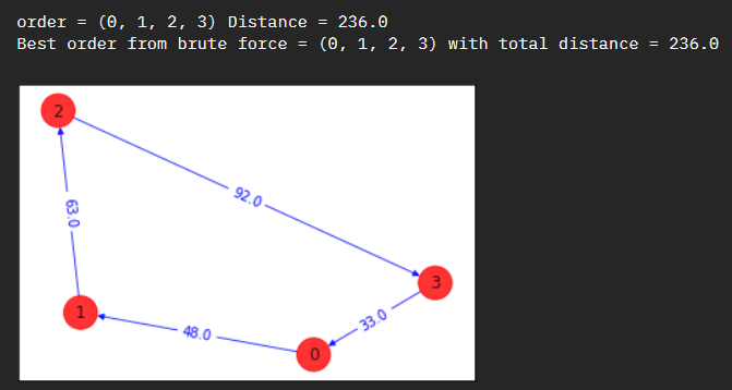
Now let’s run this on a quantum computer and see what we end up with.
# ### Specifying the backend and creating quantum instance
algorithm_globals.random_seed = 123
seed = 10598
backend = Aer.get_backend("qasm_simulator")
quantum_instance = QuantumInstance(backend, seed_simulator=seed, seed_transpiler=seed)

# ### Building an ansatz with rotational Y gates
# # We can use a traditional VQE with an ansatz, which is a trial function selected as an initial guess approximating the minimum eigenstate of a Hamiltonia, built with Y single-qubit rotations and entangler steps.
# # Please note that this is heuristic ansatz, which means that it provides you with an educated guess to help solve a problem but does not guarantee to be the most optimal answer.

spsa = SPSA(maxiter=300)
ry = TwoLocal(qubitOp.num_qubits, "ry", "cz", reps=5, entanglement="linear")
vqe = VQE(ry, optimizer=spsa, quantum_instance=quantum_instance)

result = vqe.compute_minimum_eigenvalue(qubitOp)

# ### Print solution
print("energy:", result.eigenvalue.real)
print("time:", result.optimizer_time)
x = tsp.sample_most_likely(result.eigenstate)
print("feasible:", qubo.is_feasible(x))
z = tsp.interpret(x)
print("solution:", z)
print("solution objective:", tsp.tsp_value(z, adj_matrix))
draw_tsp_solution(tsp.graph, z, colors, pos)
z = tsp.interpret(x)
print("solution:", z)
print("solution objective:", tsp.tsp_value(z, adj_matrix))
draw_tsp_solution(tsp.graph, z, colors, pos)
To add graph
Parameterized Quantum Circuits
Our QUBO example above is, by definition, unconstrained. The requirement is that the variables are binary, in the case of TSP either 1 or 0, visited or not. Most of the problems we are interested in solving will not be as simple and will include additional constraints. These constraints can be incorporated into our QUBO approach however by introducing penalties into the objective function.
We will explore this by creating a problem specific parameterized quantum circuit for our TSP problem.
The challenge explores a paper and the approach to optimizing a VQE run by focusing on breaking down the overall solution space into multiple single-solution problem spaces - corresponding to each constraint.
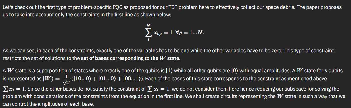
In short, since our challenge example is a 3-node graph, we can look at the solution sub-spaces in three separate groupings.
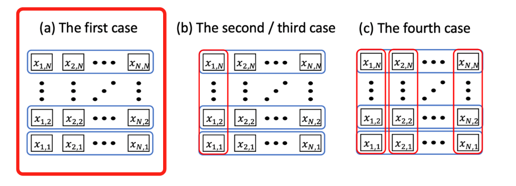
First case - W state
To start, we need to come up with a quantum circuit that generates the three qubit W-state.
from qiskit import QuantumRegister, ClassicalRegister
from qiskit.circuit import ParameterVector, QuantumCircuit

# Initialize circuit
qr = QuantumRegister(3)
cr = ClassicalRegister(3)
circuit = QuantumCircuit(qr,cr)

# Initialize Parameter with θ
theta = ParameterVector('θ', 2)

#### enter your code below ####
# Apply gates to circuit
circuit.x(0)

circuit.ry(theta[0],1)
circuit.cz(0,1)
circuit.ry(-theta[0],1)

circuit.ry(theta[1],2)
circuit.cz(1,2)
circuit.ry(-theta[1],2)

circuit.cx(1,0)
circuit.cx(2,1)

#### enter your code above ####

circuit.measure(qr,cr)
circuit.draw("mpl") 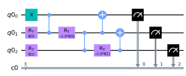
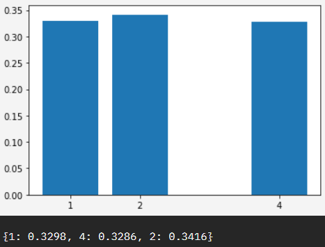
Which when run on a quantum computer we would expect 1,2,4 to be equal, or close to equal distribution - representing 001,010,100 - or our required W state.
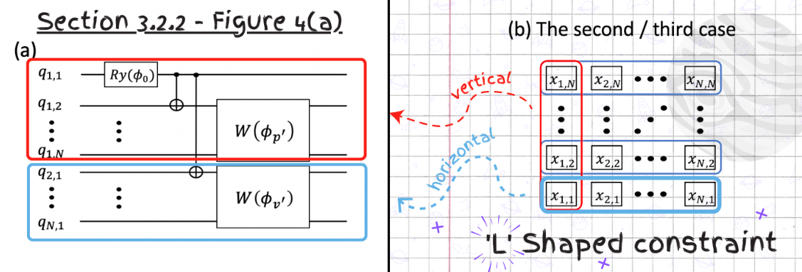
We then continue to follow the paper’s routine and build out the TSP problem’s second constraint in circuit.
Holistically, what we are trying to do is take each of the W states (total 3 states from above) and then build out each state’s solution space. In other words were are building out each hypothetical on if each W state was selected, and building it into a single quantum circuit.
Working with the W state code above, we can continue:
from qiskit import QuantumRegister, ClassicalRegister
from qiskit.circuit import ParameterVector, QuantumCircuit
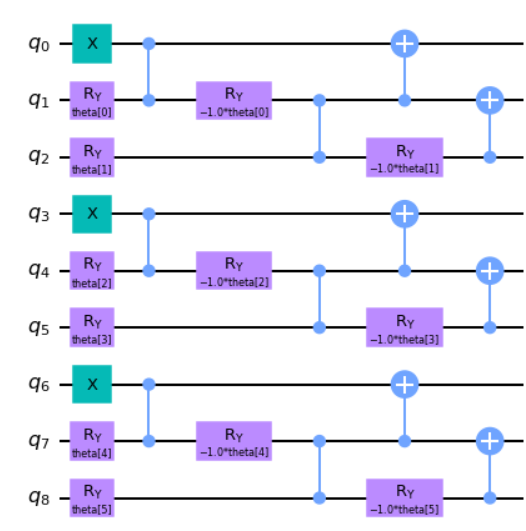
def tsp_entangler(N):
# Define QuantumCircuit and ParameterVector size
circuit = QuantumCircuit(N**2)
theta = ParameterVector('theta',length=(N-1)*N)
#############
# Hint: One of the approaches that you can go for is having an outer `for` loop for each node and 2 inner loops for each block. /
# Continue on by applying the same routine as we did above for each node with inner `for` loops for /
# the ry-cz-ry routine and cx gates. Selecting which indices to apply for the routine will be the /
# key thing to solve here. The indices will depend on which parameter index you are checking for and the current node! /
# Reference solution has one outer loop for nodes and one inner loop each for rz-cz-ry and cx gates respectively.
#############
#### enter your code above ####
#print(f'N:{N}')
for i in range(N):
# X Gate
# Parameter Gates
# CX gates
#print(f'i:{i}')
circuit.x(i*N)
for j in range(N-1):
#print(f'j:{j}')
#print(f'index:{(i*(N-1))+j}')
circuit.ry(theta[(i*(N-1))+j],(i*N)+j+1)
circuit.cz((i*N)+j,(i*N)+j+1)
circuit.ry(-theta[(i*(N-1))+j],(i*N)+j+1)
for k in range(N-1):
circuit.cx((i*N)+1+k,(i*N)+k)
#### enter your code above ####
return circuitWhich ends up looking like the following circuit for 3 constraints.
Second case - second constraint
Now that we have a good understanding of how to combine solution states on the first constraint, let’s move on to combining this with the second constraint solutions.
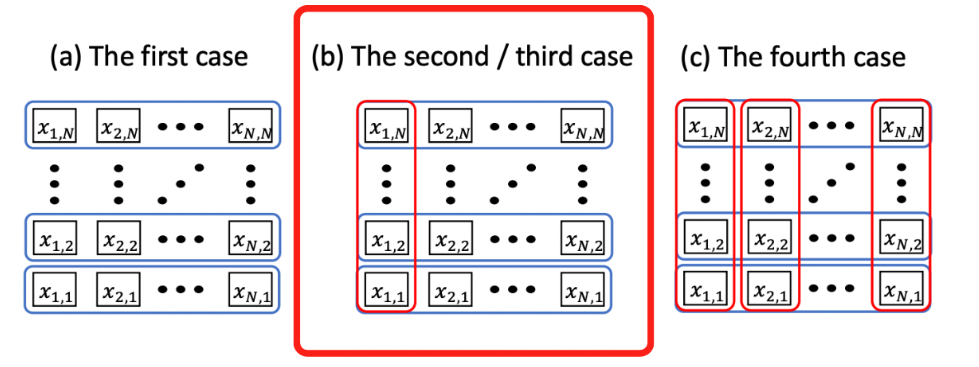
Here, unlike the first PQC, we need to add more correlations among the qubits since we will be mapping more variables across the whole matrix representation. Since we have variables that appear both in the first and second line, we can no longer realize the constraints by just tensor products. We will entangle the parametrized W gates using CNOT gates to achieve the entanglement.
Let’s start building the second PQC similarly to the first and start with defining our L-shaped constraint.
from qiskit import QuantumRegister, ClassicalRegister
from qiskit.circuit import ParameterVector, QuantumCircuit

l_circuit = QuantumCircuit(n**2)
theta = ParameterVector('theta',length=(n-1)*n-1)

# L-Shaped Entangler
l_circuit.ry(theta[0],0)
l_circuit.cx(0,1)
l_circuit.cx(0,3)

l_circuit.barrier()

#W_phi_p
l_circuit.x(1)
l_circuit.ry(theta[1],2)
l_circuit.cz(1,2)
l_circuit.ry(-theta[1],2)
l_circuit.cx(2,1)

l_circuit.barrier()

#W_phi_v
l_circuit.x(3)
l_circuit.ry(theta[2],6)
l_circuit.cz(3,6)
l_circuit.ry(-theta[2],6)
l_circuit.cx(6,3)

l_circuit.draw("mpl") 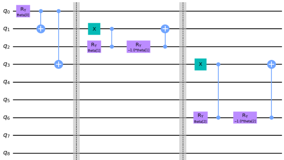
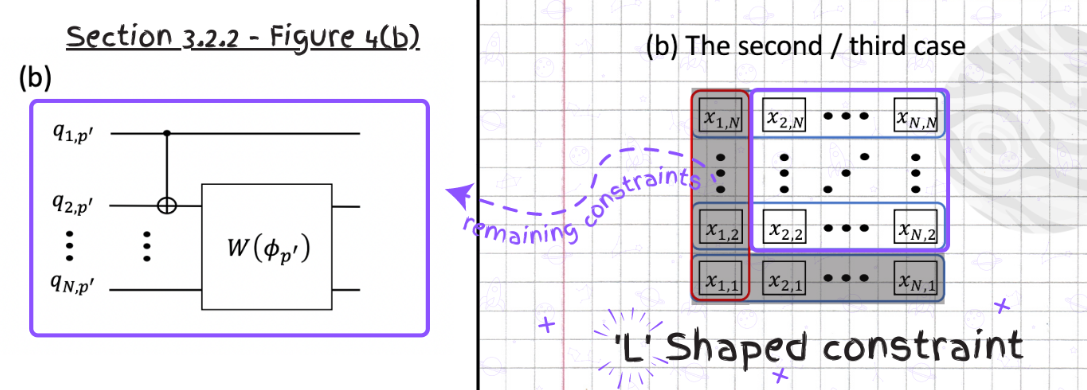
Next, we need to encode the remaining constraints excluding the ones we applied. Since the constraints for the remaining part are already determined, they can be read in a similar way as the previous problem by applying the corresponding CNOT gates followed by the parametrized W state gates on the qubits mapped variables.
from qiskit import QuantumRegister, ClassicalRegister
from qiskit.circuit import ParameterVector, QuantumCircuit

r_circuit = QuantumCircuit(n**2)
theta = ParameterVector('theta',length=(n-1)*n-1)

# Two blocks remaining for N = 3
# Block 1 ---------
r_circuit.x(4)
r_circuit.ry(theta[3],5)
r_circuit.cz(4,5)
r_circuit.ry(-theta[3],5)
r_circuit.cx(5,4)

# Block 2 ---------
r_circuit.x(7)
r_circuit.ry(theta[4],8)
r_circuit.cz(7,8)
r_circuit.ry(-theta[4],8)
r_circuit.cx(8,7)

r_circuit.draw("mpl") 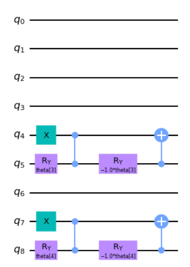
Then bridging the two sections together we get our full second constraint circuit.

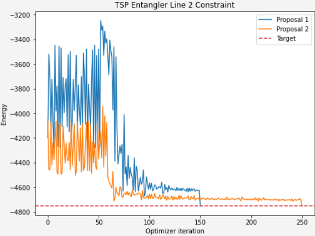
Finally, we can solve our second-constraint circuit and list out the optimized parameters.
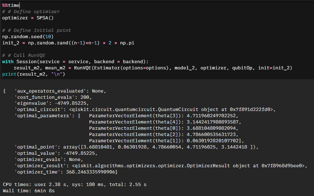
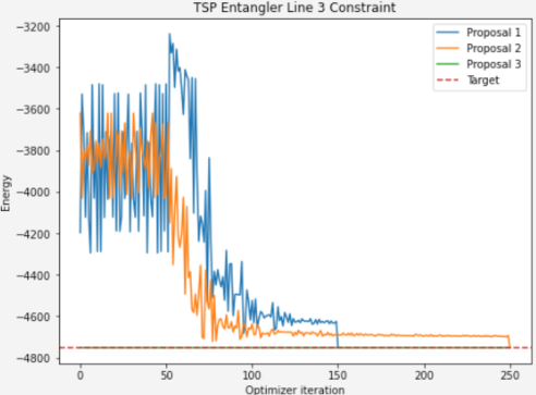
Where this gets tied all together is where we compare it to the first model in terms of convergence. We can see that the more optimized solution set converges quicker.
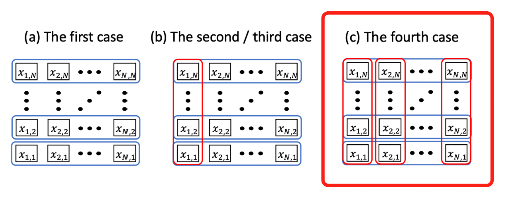
Third case - all constraints
Now we can continue and expand to all constraints. We consider all constraints to completely exclude the infeasible answers in the above image. The set of the bases of our new quantum state then includes only feasible answers. Unlike the previous two states where we saw convergence to the optimal solution, we should see here an immediate, optimal result.
We will approach this by treating the quantum circuit as a permutation matrix and recursively build on blocks we’ve already established.
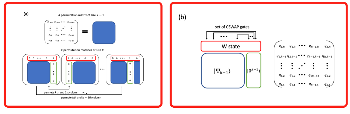
We are pointed again to the referenced paper on how to approach the solution.

Using our existing blocks and the referenced approach we can put it to code.
n = 3
model_3 = QuantumCircuit(n**2)
theta = ParameterVector('theta',length=(n-1)*n//2)

# Build a circuit when n is 2
# 2x2 in overall 3x3 structure
## (1,1 - q0)
## (1,2 - q3)
## (2,1 - q1)
## (2,2 - q4)

model_3.x(0)

model_3.ry(theta[0],1)
model_3.cz(0,1)
model_3.ry(-theta[0],1)
model_3.cx(1,0)

model_3.cx(1,3)
model_3.cx(0,4)


# Apply a parameterized W state gate
## top 'row' being:
## (1,3 - q6)
## (2,3 - q7)
## (3,3 - q8)
model_3.x(6)

model_3.ry(theta[1],7)
model_3.cz(6,7)
model_3.ry(-theta[1],7)

model_3.ry(theta[2],8)
model_3.cz(7,8)
model_3.ry(-theta[2],8)

model_3.cx(7,6)
model_3.cx(8,7)

# Apply 4 CSWAP gates
model_3.cswap(6, 2, 0)
model_3.cswap(6, 5, 3)

model_3.cswap(7, 2, 1)
model_3.cswap(7, 5, 4)

model_3.draw("mpl") 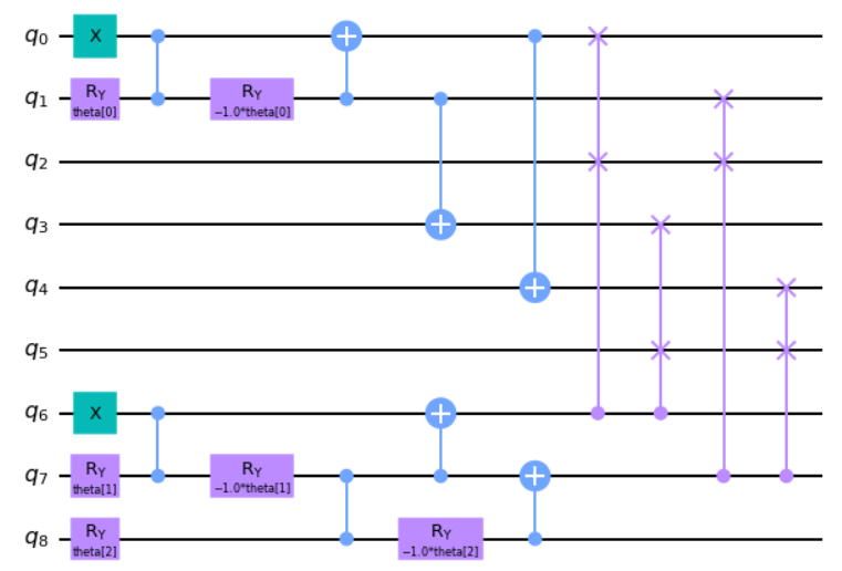
And the beauty of the circuit above is that it represents the superposition of the 6 feasible answers. Running our third model through a VQE runtime however, we can clearly see that while our first two models converged towards the right answer, the third model only represents feasible answers, so immediately starts at the minimal solution space.
Summary
In all this was a great event as usual. The cohesive narrative, and building on the exercises allowed us to experiment with the Qiskit runtime primitives in the context of a challenge many of us have seen before - namely optimization. I enjoyed the comparison of the first, second, and third model efficiencies in the optimization notebook as well, clearly illustrating the concepts of the reference paper and making it “make sense”.

Thanks folks, until next time!