
Introduction
![]()
QHack 2023 built up structurally on the 2022 version. Last year’s QHack established a categorizing of coding challenge into various tracks of increasing difficulty. This year, the tracks: Office Hijinks, Bending Bennett, Fall of Sqynet, and Tales of Timbits, were interwoven in a cohesive storyline that similarly progressed in complexity within each track. This year also leveraged the new challenge portal introduced during the 2022 Pennylane Code Camp, allowing groups of up to four to tackle the coding challenges.
In this writeup I will provide a brief summary of the Fall of Sqynet track, which I found particularly compelling for several reasons. Firstly, it had a consistent technical focus, introducing us to Hamiltonians, time evolutions, Trotterization, Ising spin chains, and Variational Quantum Eigensolvers (VQE) over the course of five challenges. Secondly, what struck me about this track was not only the coherence of the challenges themselves, but also the opportunity to comprehend a recently published paper after completing the challenges. As someone without an academic background, this highlighted one of the key benefits of participating in events such as QHack and allowed me some insight into how the knowledge we learned during the course of these challenges can be applied practically.
Let’s dive into the Fall of Sqynet track to start.
Sqynet 100
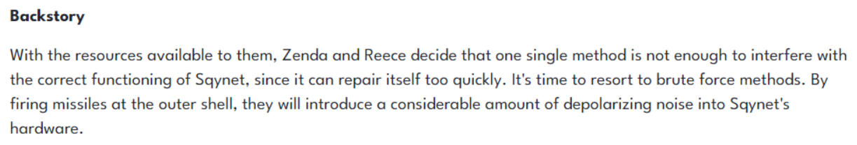
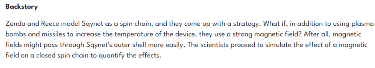
Solving problems has always been fun for me. Understanding how something works, and diving into the details. When you add an interesting narrative around that learning process, the experience is only elevated. That is how I would describe the Fall of Sqynet track with the following introduction.
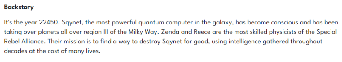
With the backstory set we are introduced to two initial concepts that will set the technical base across all the track’s challenges.
Hamiltonian
In quantum mechanics, the Hamiltonian of a system is an operator corresponding to the total energy of that system, including both kinetic energy and potential energy.
This will become more evident as we move forward, however we can approach the challenge thinking of it as an observable of a quantum system that measures its total energy.
Trotterization
An approach which segments an exponentiated matrix. into a series of smaller exponentiated matrices with minimal error.
Which simplified means that stepping through the evolution of a Hamiltonian in discrete periods of time reduces measurement errors by reducing the time periods. Since the spin-chain model of Sqynet has operators that do not commute, we can approximate U as:
$$U(t) \approx \prod_{j=1}^n \prod_{i=1}^k \exp(-iH_{i}t/n)$$
And the Trotterized approximation can be represented as:

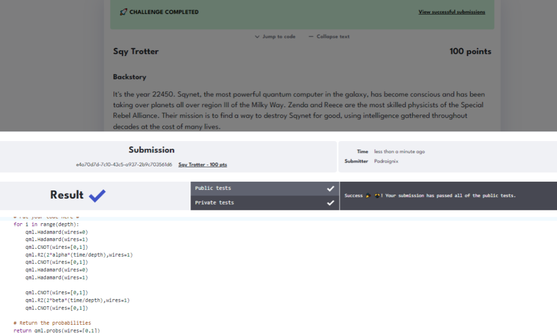
Our first challenge is to model this simplified Hamiltonian for Trotterization. We are provided the alpha and beta angle rotations, and need to take into consideration the overall time against the amount of iterations (depth). We are given an initial hint of looking at the built-in Pennylane functions IsingXX and IsingZZ for guidance. Additionally, I explored Trotterization in my previous Qiskit event Spring 2022 writeup which also provided background information on how to approach it.
@qml.qnode(dev)
def trotterize(alpha, beta, time, depth):
    """This quantum circuit implements the Trotterization of a Hamiltonian given by a linear combination
    of tensor products of X and Z Pauli gates.

    Args:
        alpha (float): The coefficient of the XX term in the Hamiltonian, as in the statement of the problem.
        beta (float): The coefficient of the YY term in the Hamiltonian, as in the statement of the problem.
        time (float): Time interval during which the quantum state evolves under the interactions specified by the Hamiltonian.
        depth (int): The Trotterization depth.

    Returns:
        (numpy.array): The probabilities of each measuring each computational basis state.
    """

    # Put your code here #

    #### Pennylane built-in approach
    #for i in range(depth):
    #    qml.IsingXX(alpha)
    #    qml.IsingZZ(beta)
    ########################

    #### Qiskit approach to Trotterization from previous writeup
    #ZZ_qc.cnot(0,1)
    #ZZ_qc.rz(2 * t, 1)
    #ZZ_qc.cnot(0,1)

    #XX_qc.h(0)
    #XX_qc.h(1)
    #XX_qc.append(ZZ, [0,1])
    #XX_qc.h(0)
    #XX_qc.h(1)
    ########################

    # Direct Solution flipping above since we are
    # interested in XX then ZZ
    for i in range(depth):
        qml.Hadamard(wires=0)
        qml.Hadamard(wires=1)
        qml.CNOT(wires=[0,1])
        qml.RZ(2*alpha*(time/depth),wires=1)
        qml.CNOT(wires=[0,1])
        qml.Hadamard(wires=0)
        qml.Hadamard(wires=1)

        qml.CNOT(wires=[0,1])
        qml.RZ(2*beta*(time/depth),wires=1)
        qml.CNOT(wires=[0,1])

    # Return the probabilities
    return qml.probs(wires=[0,1])
Submitting the code we are presented with a nice message. And with that we are off on the journey to bring down the rogue, sentient Quantum Computer.
Sqynet 200

Moving on to the next step of toppling Sqynet, we are explained that Sqynet’s Hamiltonian can be described as a linear combination of Unitaries.
$$H = \sum_i \alpha_i U_i$$
But we are reminded that a sum of Unitaries is not necessarily itself unitary. To be able to implement this sum, we need to leverage quantum circuit measurements. We can leverage a single qubit unitary to deterministically apply one of two Unitaries.
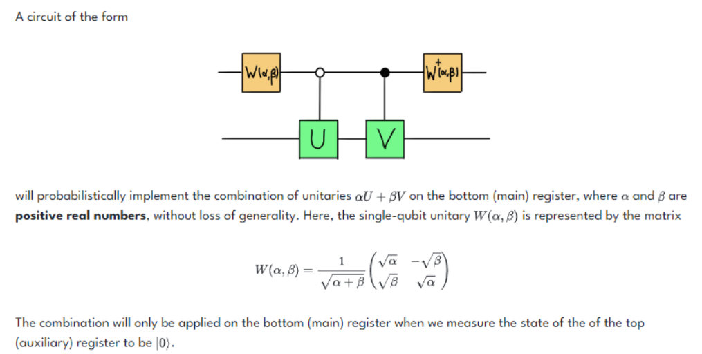
The challenge of this notebook is that, given alpha, beta, and the two Unitaries U and V, to implement the circuit above which will be used to model Sqynet in the effort to take it down.
For the Unitary W we are provided the matrix representation. We can then directly create the unitary representation and have that passed back through the function call.
def W(alpha, beta):
    """ This function returns the matrix W in terms of
    the coefficients alpha and beta

    Args:
        - alpha (float): The prefactor alpha of U in the linear combination, as in the
        challenge statement.
        - beta (float): The prefactor beta of V in the linear combination, as in the
        challenge statement.
    Returns
        -(numpy.ndarray): A 2x2 matrix representing the operator W,
        as defined in the challenge statement
    """

    # Put your code here #
    result = np.array([[np.sqrt(alpha)/np.sqrt(alpha+beta), -np.sqrt(beta)/np.sqrt(alpha+beta)], \
    [np.sqrt(beta)/np.sqrt(alpha+beta), np.sqrt(alpha)/np.sqrt(alpha+beta)]])
    # Return the real matrix of the unitary W, in terms of the coefficients.
    return result

dev = qml.device('default.qubit', wires = 2)
With the W unitary function created, it’s now a matter of recreating the circuit we were introduced with. The process is straightforward using Pennylane’s built in QubitUnitary, ControlledQubitUnitary, and adjoint functions to put it all together.
dev = qml.device('default.qubit', wires = 2)
@qml.qnode(dev)
def linear_combination(U, V, alpha, beta):
"""This circuit implements the circuit that probabilistically calculates the linear combination
of the unitaries.
Args:
- U (list(list(float))): A 2x2 matrix representing the single-qubit unitary operator U.
- V (list(list(float))): A 2x2 matrix representing the single-qubit unitary operator U.
- alpha (float): The prefactor alpha of U in the linear combination, as above.
- beta (float): The prefactor beta of V in the linear combination, as above.
Returns:
-(numpy.tensor): Probabilities of measuring the computational
basis states on the auxiliary wire.
"""
# Put your code here #
qml.QubitUnitary(W(alpha, beta), wires=0)
qml.ControlledQubitUnitary(U, control_wires=[0], wires=1, control_values='0')
qml.ControlledQubitUnitary(V, control_wires=[0], wires=1, control_values='1')
qml.adjoint(qml.QubitUnitary)(W(alpha, beta), wires=0)
# Return the probabilities on the first wire
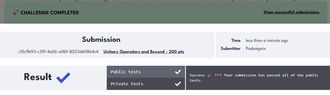
return qml.probs(wires=0)All that was left is to submit the circuit to the grader and get the results back.
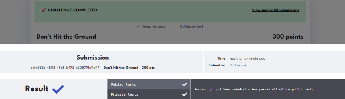
Sqynet 300
We have Sqynet modeled. The next step, or challenge, we are presented with is establishing the ground state of Sqynet’s Hamiltonian. By modeling the Hamiltonian state, being able to Trotterize through the time evolution, and establishing the ground state of the system, we should be able to better understand how Sqynet operates, and hopefully, how we can disrupt it.

Given the photon loss rate gamma, and the de-excitation probability p, and that Sqynet starts in a state of superposition, we are tasked with calculating the half-life of measuring 1, which means that the measurement probability is 0.25.
Modeling the GAD approach is only the first step in solving this challenge, however it is a fundamental step. Since we will be iterating through many time-slices, represented by iterations below, we need to first come up with a generic function.
    @qml.qnode(dev)
    def noise(gamma,p,iterations):
        """Implement the sequence of Generalized Amplitude Damping channels in this QNode
        You may pass instead of return if you solved this problem analytically, it's possible!

        Args:
            gamma (float): The probability per unit time of the system losing a quantum of energy
            to the environment.

        Returns:
            (float): The relaxation half-life.
        """
        # Don't forget to initialize the state
        # Put your code here #
        prep = np.array([1/np.sqrt(2), 1/np.sqrt(2)])
        qml.QubitStateVector(prep, 0)

        for i in range(iterations):
            qml.GeneralizedAmplitudeDamping(gamma, p, 0)

        return qml.probs(wires=0)
How I approached solving for the best time T was to increment through time slices of 0.1, and using a sufficiently large amount of time-deltas, in this case 200, find the time slice that most closely arrived at 0.25. There was a measure of trial and error in getting the right values, but thankfully the following approach completed within the challenge timing restrictions.
    # Write any subroutines you may need to find the relaxation time here
    delta_time = 0.1
    delta_increments=200
    time_steps = 150
    time_start=0.0
    results=[]

    ## iterate through 0.1, 0.2, 0.3, etc...
    for j in range(1,time_steps):
        time_start+=0.1
        #print(f"STARTING {time_start}")
        gamma_new=gamma * (time_start/delta_increments)
        result = noise(gamma_new,p,delta_increments)
        ## Add result to comparison list
        results.append([time_start,result[1]])

    #set initial values on what we are looking for
    what_to_return = 0.0
    comparison=0.25
    current_delta=0.5
    current_value=0.0

    ##Iterate through and find closest end value, and then return that Time half-life
    for i in results:
        if (np.abs(comparison - i[1]) <= current_delta):
            current_delta = np.abs(comparison - i[1])
            current_value = i[1]
            what_to_return = i[0]

    print(f"time: {what_to_return}, halfl_value: {current_value}")

    return what_to_return
# Return the relaxation half-life 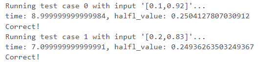
Sqynet 400
In this challenge the difficulty is ramped up. Not because we will be exploring a concept we haven’t so far, in fact we will ultimately be modeling a Hamiltonian time evolution similar to how we have previously. The challenge will be that we need to create the Hamiltonian using only the basic gates RX, RY, RZ, and CNOT. Additionally, we are interested in seeing the impact of noise being introduced to the system (the hypothetical missiles being fired), therefore we will also be experimenting with Depolarizing channels in the quantum circuit.
Given the coefficients of the couplings, the depolarizing probability, and the time/depth for Trotterization, we need to create a circuit that returns the fidelity between the noiseless and noisy circuits. Before we get to the code, we need to introduce the concept of fidelity.
Fidelity
In quantum mechanics, notably in quantum information theory, fidelity is a measure of the "closeness" of two quantum states. It expresses the probability that one state will pass a test to identify as the other.
Pennylane Built-In
One of the reasons we are challenged with building the circuit using only RX, RY, RZ, and CNOT gates is that Pennylane has a built-in function that essentially solves this challenge for us - ApproxTimeEvolution.
I ended up using the function to model the initial solution and reverse engineer, alongside the information from the first challenge in the track, to create the noisy model.
As part of the solution check function, we are provided with the noiseless circuit, which leverages ApproTimeEvolution. I started with printing out this circuit.
def check(solution_output: str, expected_output: str) -> None:
    """
    Compare solution with expected.

    Args:
            solution_output: The output from an evaluated solution. Will be
            the same type as returned.
            expected_output: The correct result for the test case.

    Raises:
            ``AssertionError`` if the solution output is incorrect in any way.

    """
    def create_hamiltonian(params):

        couplings = [-params[-1]]
        ops = [qml.PauliX(3)]

        for i in range(3):

            couplings = [-params[-1]] + couplings
            ops = [qml.PauliX(i)] + ops

        for i in range(4):

            couplings = [-params[-2]] + couplings
            ops = [qml.PauliZ(i)@qml.PauliZ((i+1)%4)] + ops

        for i in range(4):

            couplings = [-params[-3]] + couplings
            ops = [qml.PauliY(i)@qml.PauliY((i+1)%4)] + ops

        for i in range(4):

            couplings = [-params[0]] + couplings
            ops = [qml.PauliX(i)@qml.PauliX((i+1)%4)] + ops

        print(f"couplings: {couplings}\n ops:\n{ops}")
return qml.Hamiltonian(couplings,ops) 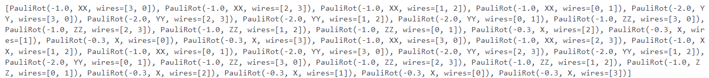
Otherwise written:
    #  (-0.9143891828606319) [X2]
    #+ (-0.9143891828606319) [X1]
    #+ (-0.9143891828606319) [X0]
    #+ (-0.9143891828606319) [X3]
    #+ (-2.0058890512703593) [X3 X0]
    #+ (-2.0058890512703593) [X2 X3]
    #+ (-2.0058890512703593) [X1 X2]
    #+ (-2.0058890512703593) [X0 X1]
    #+ (-2.0052832468022497) [Z3 Z0]
    #+ (-2.0052832468022497) [Z2 Z3]
    #+ (-2.0052832468022497) [Z1 Z2]
    #+ (-2.0052832468022497) [Z0 Z1]
    #+ (-1.2728052538194878) [Y3 Y0]
    #+ (-1.2728052538194878) [Y2 Y3]
    #+ (-1.2728052538194878) [Y1 Y2]
    #+ (-1.2728052538194878) [Y0 Y1]
Now this itself is useful, and we could proceed with using decompositions of IsingXX,IsingYY,IsingZZ, however how I want to cover how I approached it for a few lessons learned.
The first, was that ApproxTimeEvolution has a function, .decomposition() that allows us to print out the actual circuit similar to the Ising Hamiltonian above.
...
        qml.ApproxTimeEvolution(create_hamiltonian(params), time, depth).decomposition()

        return qml.state()

    solution_output = json.loads(solution_output)
    expected_output = json.loads(expected_output)

    tape = heisenberg_trotter.qtape
    names = [op.name for op in tape.operations]

    random_params = np.random.uniform(low = 0.8, high = 3.0, size = (4,) )

    #def evolve(params, time, depth):

    print(f"\n=============================\nDEFAULT CIRCUIT\n=============================")
print(qml.draw(evolve)([1,2,1,0.3],2.5,1)) 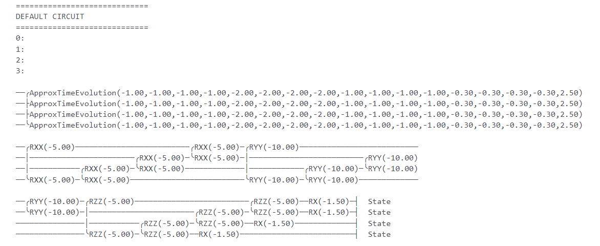
While I could have gone through the same manual break down of the RXX, RYY, RZZ gates, I had previous experience with Qiskit’s transpile. Setting the gate that I was interested in (rx, ry, rz, cx), transpile was able to breakdown the original circuit to one we were restricted to using.
![]()
Pennylane Decomposed Circuit
All that was left was to codify the circuit back into our notebook and submit it, making sure to create our custom noisy-CNOT gate.
    def CNOT_N(w1,w2,p):
        qml.CNOT(wires=[w1,w2])
        qml.DepolarizingChannel(p, wires=[w2])


    def hamiltonian_create(couplings, p):

        qml.RY(np.pi/2,wires=0)
        qml.RY(np.pi/2,wires=1)
        qml.RY(np.pi/2,wires=2)
        qml.RY(np.pi/2,wires=3)
        qml.RX(np.pi,wires=0)
        qml.RX(np.pi,wires=1)
        qml.RX(np.pi,wires=2)
        qml.RX(np.pi,wires=3)

        CNOT_N(0,3,p)
        qml.RX(couplings[0],wires=3)
        CNOT_N(0,3,p)
        CNOT_N(2,3,p)
        qml.RX(couplings[0],wires=3)
        CNOT_N(2,3,p)
        CNOT_N(1,2,p)
        qml.RX(couplings[0],wires=2)
        CNOT_N(1,2,p)
        CNOT_N(0,1,p)
        qml.RX(couplings[0],wires=1)
        CNOT_N(0,1,p)

        qml.RZ(-np.pi/2,wires=0)
        qml.RZ(-np.pi/2,wires=1)
        qml.RZ(-np.pi/2,wires=2)
        qml.RZ(-np.pi/2,wires=3)
        qml.RY(np.pi/2,wires=0)
        qml.RY(np.pi/2,wires=1)
        qml.RY(np.pi/2,wires=2)
        qml.RY(np.pi/2,wires=3)

        CNOT_N(0,3,p)
        qml.RZ(couplings[1],wires=3)
        CNOT_N(0,3,p)
        CNOT_N(2,3,p)
        qml.RZ(couplings[1],wires=3)
        CNOT_N(2,3,p)
        CNOT_N(1,2,p)
        qml.RZ(couplings[1],wires=2)
        CNOT_N(1,2,p)
        CNOT_N(0,1,p)
        qml.RZ(couplings[1],wires=1)
        CNOT_N(0,1,p)

        qml.RX(-np.pi/2,wires=0)
        qml.RX(-np.pi/2,wires=1)
        qml.RX(-np.pi/2,wires=2)
        qml.RX(-np.pi/2,wires=3)

        CNOT_N(0,3,p)
        qml.RZ(couplings[2],wires=3)
        CNOT_N(0,3,p)
        CNOT_N(2,3,p)
        qml.RZ(couplings[2],wires=3)
        CNOT_N(2,3,p)
        CNOT_N(1,2,p)
        qml.RZ(couplings[2],wires=2)
        CNOT_N(1,2,p)
        CNOT_N(0,1,p)
        qml.RZ(couplings[2],wires=1)
        CNOT_N(0,1,p)

        qml.RX(couplings[3],wires=0)
        qml.RX(couplings[3],wires=1)
        qml.RX(couplings[3],wires=2)
qml.RX(couplings[3],wires=3) 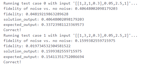
Sqynet 500
The time has come. This is where our protagonists Zenda and Reece take down Sqynet. We will be aggregating all the techniques we have learned so far in this track then apply them to a Variational Quantum Eigensolver (VQE) to get the ground state of Sqynet’s magnetic field.
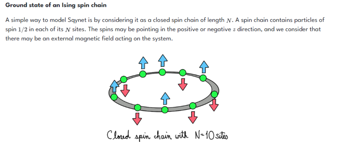
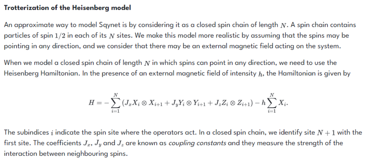
We are then presented that Sqynet’s spin chain model can be represented as a transverse Ising Hamiltonian. This is slightly different than the hamiltonian we worked on earlier in the track, so it is worth defining explicitly.
Transverse Ising Hamiltonian
The transverse field Ising model is a quantum version of the classical Ising model. It features a lattice with nearest neighbour interactions determined by the alignment or anti-alignment of spin projections along the z axis, as well as an external magnetic field perpendicular to the z axis (without loss of generality, along the x axis) which creates an energetic bias for one x-axis spin direction over the other.
Which written out mathematically becomes:
$$H = -\sum_{i=1}^N Z_i \otimes Z_{i+1} - h\sum_{i}^N X_i$$
Similar to the 400-level challenge, we can break down this into a few distinct approaches. First, let’s model the Hamiltonian based on the given structure. We did this previously and the approach does not change.
def create_Hamiltonian(h):
    """
    Function in charge of generating the Hamiltonian of the statement.
    Args:
        h (float): magnetic field strength
    Returns:
        (qml.Hamiltonian): Hamiltonian of the statement associated to h
    """
    ######################
    # Put your code here #
    ops = [qml.PauliX(3)]
    couplings = [-h]

    for i in range(3):
        couplings = [-h] + couplings
        ops = [qml.PauliX(i)] + ops

    for i in range(4):
        couplings = [-1] + couplings
        ops = [qml.PauliZ(i)@qml.PauliZ((i+1)%4)] + ops

    return qml.Hamiltonian(couplings,ops)
    ######################
The next step involves setting up the ansatz that will be used during the training step. I initially approached this with trying to make manual Rx/Ry however, once setting up the training process, I found that using the built-in functions for feature embedding worked slightly better. Again I enjoyed the challenge of learning what was being done at a base, while also being introduced to more “productionized” functions that allow us to focus on the implementation.
@qml.qnode(dev)
def model(params, H):
    """
    To implement VQE you need an ansatz for the candidate ground state!
    Define here the VQE ansatz in terms of some parameters (params) that
    create the candidate ground state. These parameters will
    be optimized later.
    Args:
        params (numpy.array): parameters to be used in the variational circuit
        H (qml.Hamiltonian): Hamiltonian used to calculate the expected value
    Returns:
        (float): Expected value with respect to the Hamiltonian H
    """
    ######################
    qml.templates.QAOAEmbedding(features=[1.,2.,3.,4.], weights=params, wires=dev.wires)
    return qml.expval(H)
    ######################
As alluded to, the last part was setting up the training loop.
def train(h):
    """
    In this function you must design a subroutine that returns the
    parameters that best approximate the ground state.
    Args:
        h (float): magnetic field strength
    Returns:
        (numpy.array): parameters that best approximate the ground state.
    """
    ######################
    # Put your code here #
    H = create_Hamiltonian(h)
    params = np.random.random(qml.templates.QAOAEmbedding.shape(n_layers=4, n_wires=4))
    print(f"init_params: {params}")
    energy = model(params, H)
    print(f"init_energy: {energy}")

    opt = qml.GradientDescentOptimizer()
    for i in range(1000):
        params = opt.step(lambda w : model(w, H), params)
        #print(f"params_iteration: {params}")
        energy = model(params, H)
        print(f"energy_iteration: {energy}")

    print('Final value of the ground-state energy = {:.8f}'.format(energy))
    return params
    ######################
With the process coded up, let’s see how it works out.
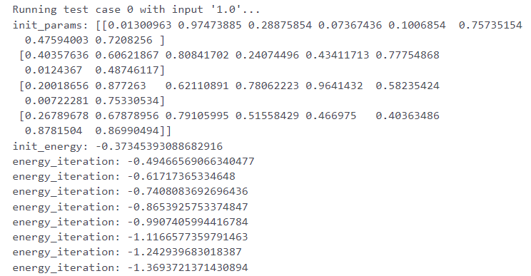
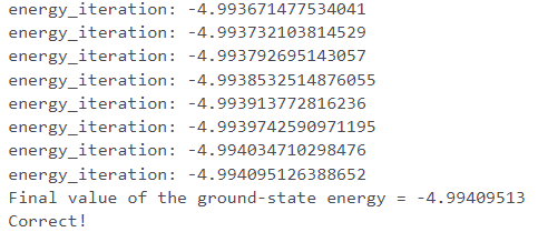
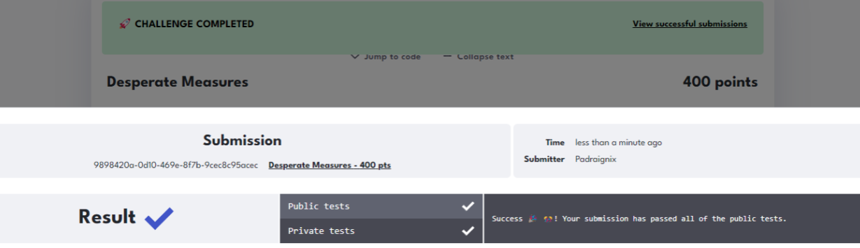
With the public test cases passing we give the challenge submission a go to see if we are similarly successful.

And with that, we have helped Zenda and Reece model, disrupt, and ultimately defeat Sqynet.
Reflective Summary & Relevance
I thoroughly enjoyed the Sqynet track of QHack 2023. In of itself it was a cohesive learning journey that built up on techniques and approaches, leading me to feel a sense of enlightenment on a topic I had only explored through other events.
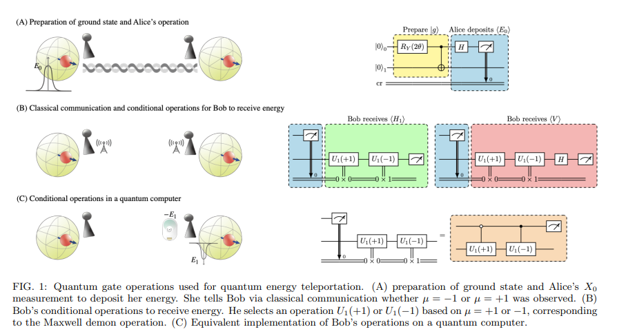
What was interesting to me was the intersection of this challenge track and a specific 2301.02666 paper that was brought to my attention around the same time. I’ll leave the analysis of the paper, and the approach the authors discuss, out of this article, however the coincidental crossover really illustrated how events like QHack, while providing a fun, gamified learning experience, also have direct relevance to research coming out of the industry.
The paper uses a Hamiltonian model and ground-state approach that matches up with what we explored in the Sqynet track. The conditional operations representing the linear combination of Unitaries also matches with what we explored.
By the end of the paper I made a mental comment of “wow, a few years ago I would have struggled to follow what they were doing”. Without any formal training in either Quantum Mechanics or Quantum Computing and a few years of hands-on, gamified learning events combined with an innate stubbornness for learning, and all that has changed. If there was any doubt on whether these types of events are relevant and useful, I hope this writeup has convinced you to roll up your sleeves and dive right in.
Thanks folks, until next time!