QHack 2021 - Circuit Training Track

Introduction

QHACK 2021 was a virtual conference hosted by Xanadu where individuals had an opportunity to learn hands on about Quantum Machine Learning. The event included a two part Hackathon for individuals to challenge themselves as well as compete against other participants around the globe. The first portion of the event included academic challenges for teams to complete for "power ups" (AWS credits and bonuses) that could be applied on the second portion which was a more creative project based effort.

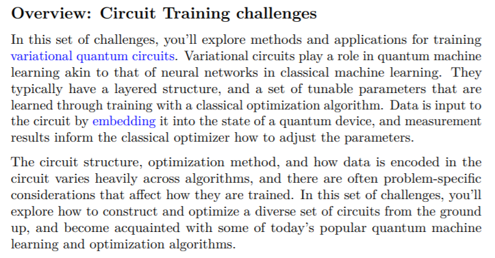
The challenges in the first portion were broken up into four categories - simple circuits, quantum gradients, circuit training, and variational quantum eigensolvers (VQE). The full challenge notebooks are still available on Xanadu's github page for anyone interested in taking a look at the original problem material. As we were competing in a team (Quantum-plators) we broke up the challenges amongst our team members and I ended up taking on the circuit training track - which included 100, 200 and 500 point challenges.

Over the course of this post I will cover my approaches and solutions to all three challenges. The first two focused more on theoretical application, ensuring we understood the fundamentals of Pennylane and QML in general. The training_circuit500 problem dove a bit deeper however, allowing us to define our own variational quantum circuit on the way to training the model with our given test data. We needed to define the circuit and properly classify hidden test data to a narrow acceptance tolerance on the hackathon portal for the submission to be successful.

Considering I had an extremely limited exposure to QML (and ML in general) prior to this event I am happy to say I managed to learn quite a bit going through these challenges and am even happier to say I was able to solve them. These events are an excellent opportunity to step outside our normal bounds in a structured format helping guide "where to start" with an element of competitiveness that allows us to push further. Without further ado, let's get to the code.

Training Circuit 100

Let's start by reading the problem statements carefully.

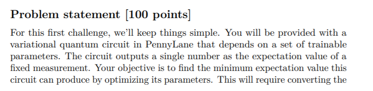
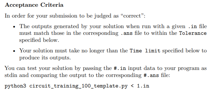
Alright let us break this down. We are given a template python file, where the challenge will be to fill in the missing sections, a pair of input and corresponding "correct" outputs to validate our code, and finally the specifications we must adhere to.

Time to take a look at the template they provided. Thankfully the organizers clearly delineated code sections we were to fill in with # QHACK # to avoid confusion. It may seem like a triviality, however small things like this marker make the challenges much clearer to participants - kudos! According to the template our variational circuit is already defined for us and the focus of this challenge is to fill in the circuit optimization portion.

def optimize_circuit(params):
    """Minimize the variational circuit and return its minimum value.
    The code you write for this challenge should be completely contained within this function
    between the # QHACK # comment markers. You should create a device and convert the
    variational_circuit function into an executable QNode. Next, you should minimize the variational
    circuit using gradient-based optimization to update the input params. Return the optimized value
    of the QNode as a single floating-point number.
    Args:
        params (np.ndarray): Input parameters to be optimized, of dimension 30
    Returns:
        float: the value of the optimized QNode
    """

    optimal_value = 0.0

    # QHACK #

    # Initialize the device
    # dev = ...

    # Instantiate the QNode
    # circuit = qml.QNode(variational_circuit, dev)

    # Minimize the circuit

    # QHACK #

    # Return the value of the minimized QNode
    return optimal_value

Everything we need to know for this first challenge is available at the Pennylane Qubit Rotation Tutorial. From first creating the Qnode, calculating the quantum gradient, to optimizing the cost/parameters, all the components are broken out and explained. In essence what we are attempting to do is run our circuit, starting with "random" parameters. The optimization algorithm will then adjust those paramaters in an attempt to find the combinations that produce the lowest "cost" as defined by our cost function. Between the challenge template and tutorial we are able to plug in the required parts and see the optimization in action.

def optimize_circuit(params):
    """Minimize the variational circuit and return its minimum value.
    The code you write for this challenge should be completely contained within this function
    between the # QHACK # comment markers. You should create a device and convert the
    variational_circuit function into an executable QNode. Next, you should minimize the variational
    circuit using gradient-based optimization to update the input params. Return the optimized value
    of the QNode as a single floating-point number.
    Args:
        params (np.ndarray): Input parameters to be optimized, of dimension 30
    Returns:
        float: the value of the optimized QNode
    """

    optimal_value = 0.0

    # QHACK #

    # Initialize the device
    # dev = ...
    dev = qml.device("default.qubit", wires=WIRES)
    # Instantiate the QNode
    circuit = qml.QNode(variational_circuit, dev)
    
    # initialise the optimizer
    steps = 50
    opt = qml.GradientDescentOptimizer(stepsize=0.4) 

    # Minimize the circuit
    for i in range(steps):
        # update the circuit parameters after each step relative to cost & params
        params = opt.step(circuit, params)
    optimal_value = circuit(params)
    # QHACK #

    # Return the value of the minimized QNode
    return optimal_value

All that is left is to run it with our provided test data and compare the output with the expected answers. Sure enough it looks good and we can submit the code to the hackathon dashboard.

Training Circuit 200

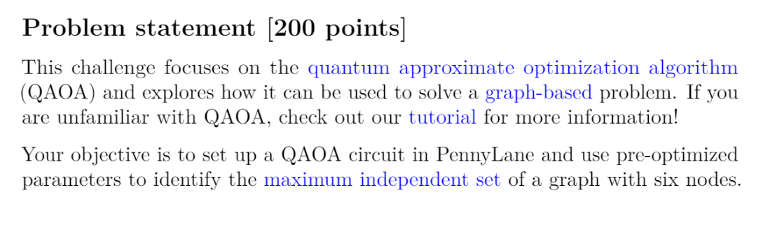
No time to rest as we still have two more challenges to tackle! This second challenge focused on quantum approximate optimization algorithm (QAOA) and solving a graph max independent problem. More specifically the problem statement.

As I had no previous experience with QAOA I gladly took a look at the suggested Pennylane QAOA Introduction.

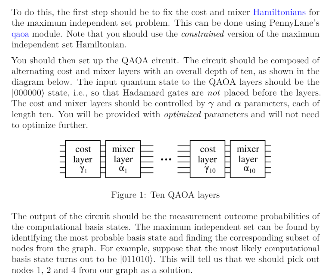
Starting with the absolute basics in the tutorial I learned how we can think of quantum circuits in terms of Hamiltonians. More specifically time evolution operators \(U(H,t) = e^{iγH}\) where γ is a scalar and \(H\) is a Hermitian operator interpreted as a Hamiltonian. The challenge problem statement referred to an optimized γ that is provided, therefore we are on the right track. There is more theory to understand before we can start coding though. As we are told that we would need to alternate 10 variants of Cost and Mixer Hamiltonians the Pennlyane QAOA tutorial covers a useful function we will be using - layers. By using this function we are able to define the initial circuit template and copy that section multiple times with ease.

At this point we are ready to start defining the QAOA code. The tutorial breaks the overall QAOA approach we need to emulate down to 6 steps.

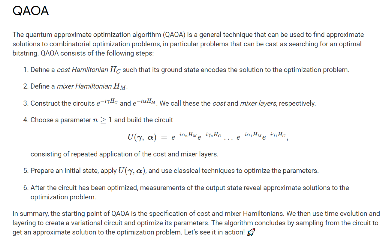
Let's see it in action indeed! The tutorial then continued with a minimum vertex cover problem, however our challenge problem is slightly different. We are looking to solve a maximum independent set of a graph with 6 nodes. We can print out the problem's graph provided in the sample data to have a better visual of what we are working with.

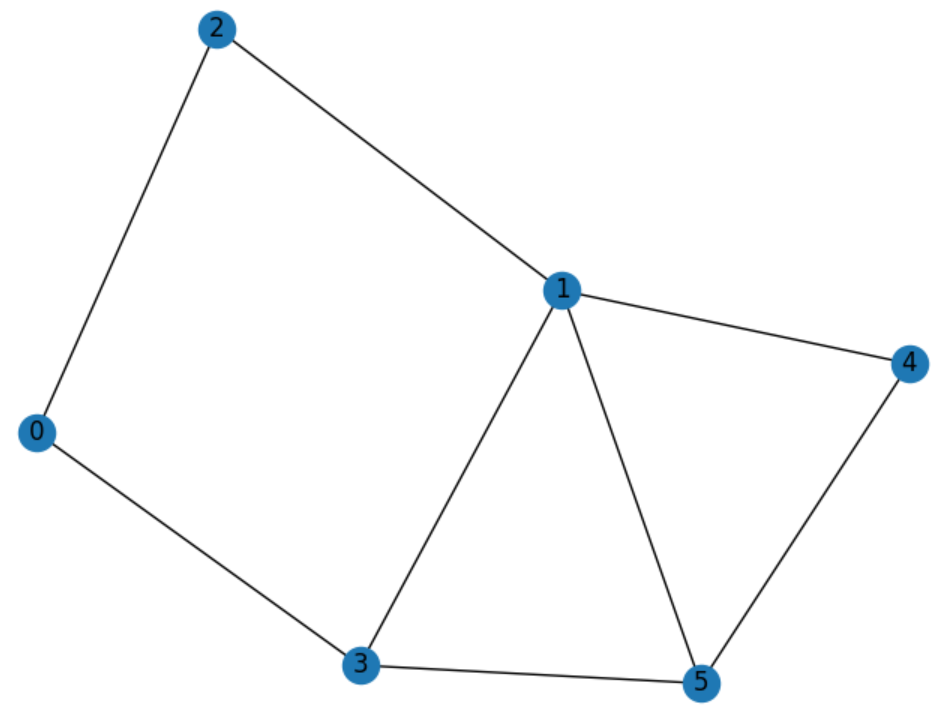
Just by looking at the graph we can tell that the answer in this case would be [2,3,4]. This is also confirmed by looking at the sample output provided. Alright we have the base information required so let's get this created.

The first part of code that we need to import is the qaoa functionality from pennylane. With that we can define our Cost and Mixer Hamiltonians.

def find_max_independent_set(graph, params):
    """Find the maximum independent set of an input graph given some optimized QAOA parameters.
    The code you write for this challenge should be completely contained within this function
    between the # QHACK # comment markers. You should create a device, set up the QAOA ansatz circuit
    and measure the probabilities of that circuit using the given optimized parameters. Your next
    step will be to analyze the probabilities and determine the maximum independent set of the
    graph. Return the maximum independent set as an ordered list of nodes.
    Args:
        graph (nx.Graph): A NetworkX graph
        params (np.ndarray): Optimized QAOA parameters of shape (2, 10)
    Returns:
        list[int]: the maximum independent set, specified as a list of nodes in ascending order
    """

from pennylane import qaoa
wires = range(6)
cost_h, mixer_h = qaoa.max_independent_set(graph, constrained=True)

The next portion follows the path of the tutorial. We need to define our template circuit and then layer it the amount of times we need - in this case ten.

def qaoa_layer(gamma, alpha):
    qaoa.cost_layer(gamma, cost_h)
    qaoa.mixer_layer(alpha, mixer_h)

def circuit1(params, **kwargs):
    qml.layer(qaoa_layer, N_LAYERS, params[0], params[1])

The last part is to create the remainder of the circuit definition and pull out the max solution of probabilities. Since we've been told that there is only a single solution per graph this ensures that the right combination is always chosen.

def probability_circuit(params):
    circuit1(params)
    return qml.probs(wires=wires)

dev = qml.device("default.qubit", wires=6)
circuit = qml.QNode(probability_circuit, dev)
probs = circuit(params)
solution = np.max(probs)
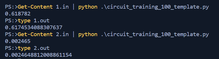
result = np.where(probs == np.amax(probs))

Let's run the code against our first input and see where we are at.

Hum...that doesn't seem right. But wait! If we convert 14 to Binary we get 001110 (reverse ordering) which translates to the 2nd, 3rd, and 4th nodes being 1 - or in quantum terms, our qubits representing the nodes of the solution. Ok so the logic works, but we need to massage the output a bit. Quickly writing a small utility that can be inserted to the code I was able to get that done. I'm sure there were much simpler ways to get this portion done, however as this wasn't the focus of the challenge I just "made it work" rather than look for an elegant solution.

test = result[0].item()
def get_bin(x, n=0):
    return format(x, 'b').zfill(n)

test_format = get_bin(test,6)
string_ans = test_format

i = 0
for char in string_ans:
    if char == "1":
        max_ind_set.append(i)
    i+=1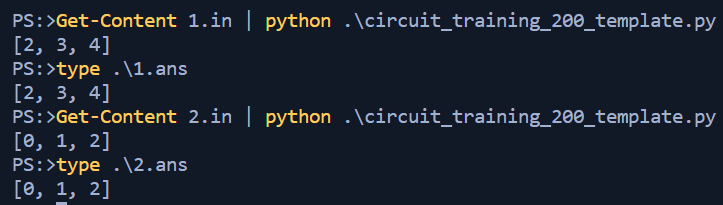  

With the code successul in terms of the test data it was uploaded to the hackathon dashboard and thankfully the hidden data-set was also evaluated properly. Two challenges down, one to go!

Training Circuit 500

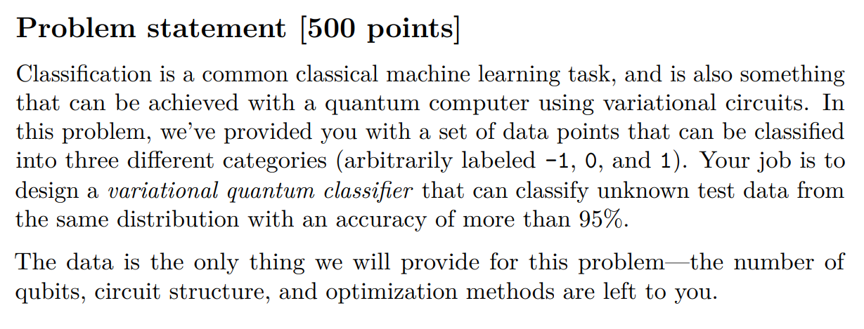
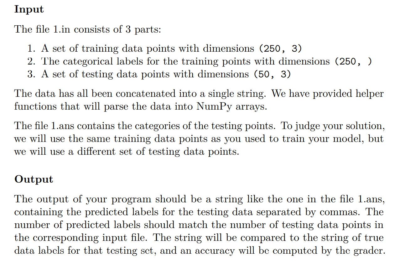
Now time to get into the beefier of the challenges! In this problem we are provided with a data set of 250 points in 3d space and their corresponding labels among [-1,0,1]. Additionally we are provided with a smaller data set of 50 points and the corresponding labels as answers. Our challenge is to create a variational quantum classifier that can properly classify the smaller test data set (where the "answer" should match the provided smaller set of 50 labels) within the stipulated time and accuracy tolerances.

As with the first two challenges there was some good Variational Classifier tutorial documentation available from Pennylane that helped get a base understanding of what we need to do. Unlike the previous two challenges however this one was not as hand holding and required us to come up with our own modifications.

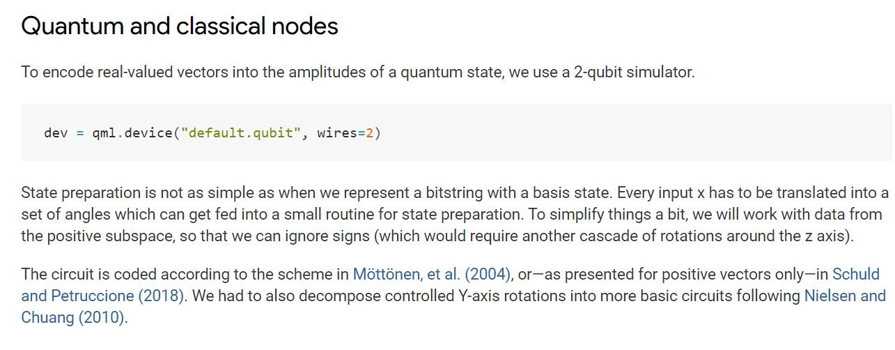
There were a couple points here that ended tripping me up in the longer run. The first is that I interpreted the translated set of angles as absolutely required in my future approach. As we will see this was not required and working with normalized data was enough to succeed. The second is that the example provided in the tutorial deals only with positive vectors. I initially went down the road of using the reference material to define my statepreparation for positive & negative space, however that ended up not being required and using the simplified, postive vector only model was successful.

Following the tutorial I first loaded in the data and prepared it for training.

def classify_data(X_train, Y_train, X_test):
    """Develop and train your very own variational quantum classifier.

    Use the provided training data to train your classifier. The code you write
    for this challenge should be completely contained within this function
    between the # QHACK # comment markers. The number of qubits, choice of
    variational ansatz, cost function, and optimization method are all to be
    developed by you in this function.

    Args:
        X_train (np.ndarray): An array of floats of size (250, 3) to be used as training data.
        Y_train (np.ndarray): An array of size (250,) which are the categorical labels
            associated to the training data. The categories are labeled by -1, 0, and 1.
        X_test (np.ndarray): An array of floats of (50, 3) to serve as testing data.

    Returns:
        str: The predicted categories of X_test, converted from a list of ints to a
            comma-separated string.
    """

    # Use this array to make a prediction for the labels of the data in X_test
    predictions = []

    # QHACK #

    ...

    X = X_train
    # pad the vectors with constant values
    padding = 0.3 * np.ones((len(X), 1))
    X_pad = np.c_[np.c_[X, padding], np.zeros((len(X), 1))]

    # normalize each input
    normalization = np.sqrt(np.sum(X_pad ** 2, -1))
    X_norm = (X_pad.T / normalization).T

    # angles for state preparation are new features
    # ultimate this wasn't required
    features = np.array([get_angles(x) for x in X_norm])
    
    Y = Y_train
    
    ####### Mapping Test Data ##########
    X_data = X_test

    # pad the vectors with constant values
    x_padding = 0.3 * np.ones((len(X_data), 1))
    X_data_pad = np.c_[np.c_[X_data, x_padding], np.zeros((len(X_data), 1))]

    # normalize each input
    x_normalization = np.sqrt(np.sum(X_data_pad ** 2, -1))
    X_data_norm = (X_data_pad.T / x_normalization).T

    # angles for state preparation are new features
    # ultimately wasn't required
    x_features = np.array([get_angles(x) for x in X_data_norm])

At this point we have X as our training data, Y as our training answers, and X_data as our testing data that we can use to validate our training model. With one more piece of code we can visualize what our data looks like at the moment.

    import matplotlib.pyplot as plt

    plt.figure()
    plt.scatter(X[:, 0][Y == 1], X[:, 1][Y == 1], c="b", marker="o", edgecolors="k")
    plt.scatter(X[:, 0][Y == 0], X[:, 1][Y == 0], c="g", marker="o", edgecolors="k")
    plt.scatter(X[:, 0][Y == -1], X[:, 1][Y == -1], c="r", marker="o", edgecolors="k")
    plt.title("Original data")
    plt.show()

    plt.figure()
    dim1 = 0
    dim2 = 1
    plt.scatter(
        X_norm[:, dim1][Y == 1], X_norm[:, dim2][Y == 1], c="b", marker="o", edgecolors="k"
    )
    plt.scatter(
        X_norm[:, dim1][Y == -1], X_norm[:, dim2][Y == -1], c="r", marker="o", edgecolors="k"
    )
    plt.scatter(
        X_norm[:, dim1][Y == 0], X_norm[:, dim2][Y == 0], c="g", marker="o", edgecolors="k"
    )
    plt.title("Padded and normalised data (dims {} and {})".format(dim1, dim2))
    plt.show()

    plt.figure()
    dim1 = 0
    dim2 = 1
    plt.scatter(
        features[:, dim1][Y == 1], features[:, dim2][Y == 1], c="b", marker="o", edgecolors="k"
    )
    plt.scatter(
        features[:, dim1][Y == -1], features[:, dim2][Y == -1], c="r", marker="o", edgecolors="k"
    )
    plt.scatter(
        features[:, dim1][Y == 0], features[:, dim2][Y == 0], c="g", marker="o", edgecolors="k"
    )
    plt.title("Feature vectors (dims {} and {})".format(dim1, dim2))
    plt.show()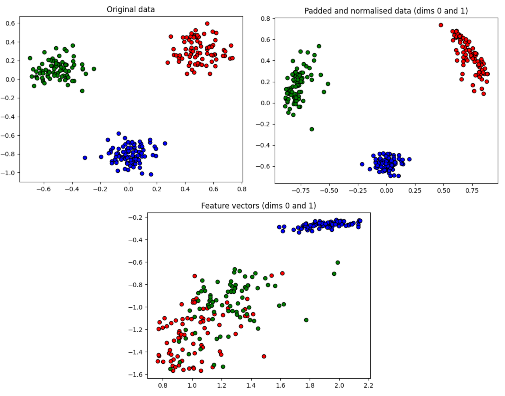

As we can see from the graph, which unfortunately wasn't immediately clear for me at the time, the normalized data has the best distribution for classifying the data. Call it fog of competition but only once I came up for a breath and took a step back after beating my head against training with the feature map data did I realize this.

Before we can take a stab at classifying the data itself there are still some functions to define. We still need to create the circuits, the cost functions, the state preparation circuit, and an ability to define whether a prediction was accurate or not.

    n_qubits = 2
    dev = qml.device("default.qubit", wires=n_qubits)

    def layer(W):
        qml.Rot(W[0, 0], W[0, 1], W[0, 2], wires=0)
        qml.Rot(W[1, 0], W[1, 1], W[1, 2], wires=1)
        qml.CNOT(wires=[0, 1])
    
    def get_angles(x):

        beta0 = 2 * np.arcsin(np.sqrt(x[1] ** 2) / np.sqrt(x[0] ** 2 + x[1] ** 2 + 1e-12))
        beta1 = 2 * np.arcsin(np.sqrt(x[3] ** 2) / np.sqrt(x[2] ** 2 + x[3] ** 2 + 1e-12))
        beta2 = 2 * np.arcsin(np.sqrt(x[2] ** 2 + x[3] ** 2)/ np.sqrt(x[0] ** 2 + x[1] ** 2 + x[2] ** 2 + x[3] ** 2))

        return np.array([beta2, -beta1 / 2, beta1 / 2, -beta0 / 2, beta0 / 2])

    def statepreparation(a):

        # In theory this only works with positive numbers
        qml.RY(a[0], wires=0)

        qml.CNOT(wires=[0, 1])
        qml.RY(a[1], wires=1)
        qml.CNOT(wires=[0, 1])
        qml.RY(a[2], wires=1)

        qml.PauliX(wires=0)
        qml.CNOT(wires=[0, 1])
        qml.RY(a[3], wires=1)
        qml.CNOT(wires=[0, 1])
        qml.RY(a[4], wires=1)
        qml.PauliX(wires=0)

    @qml.qnode(dev)
    def circuit(weights, angles):
        statepreparation(angles)
        for W in weights:
            layer(W)
        return qml.expval(qml.PauliZ(1))

    def variational_classifier(var, angles):
        weights = var[0]
        bias = var[1]
        return circuit(weights, angles) + bias
    
    def square_loss(labels, predictions):
        loss = 0
        for l, p in zip(labels, predictions): 
            loss = loss + (l - p) ** 2
        loss = loss / len(labels)
        return loss
    
    def accuracy(labels, predictions):
        loss = 0
        for l, p in zip(labels, predictions):
            if abs(l - p) < 1e-3:
                loss = loss + 1
        loss = loss / len(labels)
        return loss

    def correct_labels(predictions):
        correct_label = []
        for p in predictions:
            if p < -0.3:
                correct_label.append(-1)
            elif p > 0.3:
                correct_label.append(1)
            else:
                correct_label.append(0)
        return correct_label

    def cost(weights, features, labels):
        predictions = [variational_classifier(weights, f) for f in features]
        return square_loss(labels, predictions)

The main thing to note is the correct_labels function. This is an important portion that required tweaking for the model to work. In hindsight one can see from the normalized graph above how a prediction value hinging at +/- 0.3 would cleanly delineate our three categories. With the original data, there is a slight cross over that would end up polluting our predictions, and with the attempted feature map it would address one category while not working well for the other two.

With all the components ready we can create the training loop and see if we are able to hit our tolerances.

    np.random.seed(1337)
    num_data = 250
    num_train = 50
    index = np.random.permutation(range(num_data))
    feats_train = X_norm
    feats_val = X_data_norm
    #Hardcode "1.ans" for training comparison
    Y_val = [1,0,-1,0,-1,1,-1,-1,0,-1,1,-1,0,1,0,-1,-1,0,0,1,1,0,-1,0,0,-1,0,-1,0,0,1,1,-1,-1,-1,0,-1,0,1,0,-1,1,1,0,-1,-1,-1,-1,0,0]

    num_qubits = 2
    num_layers = 6
    var_init = (0.01 * np.random.randn(num_layers, num_qubits, 3), 0.0)

    opt = NesterovMomentumOptimizer(0.1)
    batch_size = 5

    var = var_init

    for it in range(50):

        # Update the weights by one optimizer step
        batch_index = np.random.randint(0, num_train, (batch_size,))

        feats_train_batch = feats_train[batch_index]
        Y_train_batch = Y_train[batch_index]
        var = opt.step(lambda v: cost(v, feats_train_batch, Y_train_batch), var)
        
        # Compute predictions on train and validation set
        predictions_train_bad = [variational_classifier(var, f) for f in feats_train]
        predictions_train = correct_labels(predictions_train_bad)
        #predictions_val = [variational_classifier(var, f) for f in feats_val]
        predictions_val_bad = [variational_classifier(var, f) for f in feats_val]
        predictions_val = correct_labels(predictions_val_bad)

        # Compute accuracy on train and validation set
        acc_train = accuracy(Y_train, predictions_train)
        acc_val = accuracy(Y_val, predictions_val)

        print(
            "Iter: {:5d} | Cost: {:0.7f} | Acc train: {:0.7f} | Acc validation: {:0.7f} "
            "".format(it + 1, cost(var, X_norm, Y), acc_train, acc_val)
        )
        
    predictions_val_bad = [variational_classifier(var, f) for f in feats_val]
    predictions = correct_labels(predictions_val_bad)
    # QHACK #

    return array_to_concatenated_string(predictions)

You'll notice I included a print statement within the loop. This was used during the testing period to help adjust where required and ultimately commented out for the submission. Additionally I did play around with a few different optimizers, however there was no deeper analysis done between the different types and ultimately the NesterovMomentumOptimizer approach is what I stayed with in the end.

While in reality there were many back and forths between execution and tweaking, let's pretend we don't know the outcome yet and see how the loop responds.

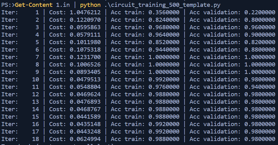
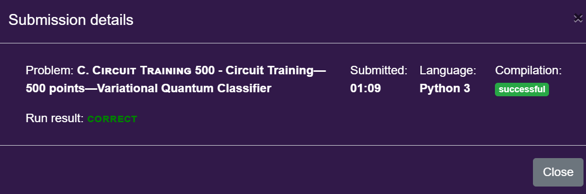
Well that seems within our tolerance of 96% alright! The last part was to ensure the processing is completed with 60 seconds, and clean up the output to only spit out the prediction list. I arbitrarily chose 8 iterations since iterations 7,8,9 all returned 100% accuracy and figure why not aim for the middle of that pile since the processing time to that point was well within 60 seconds. A few comments later I reran the script and compared it against output.

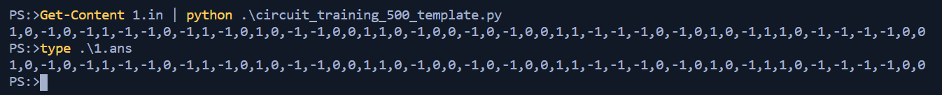
That is looking good! The final step was to upload the code and hope that it behaves similarly with the hidden test data. Thankfully within a few minutes of submitting I was greeted with a welcomed message.

And thus the chapter ended for the training circuit track.

Conclusion & Recap

With the rest of my team we were able to claim a few more victories early and enjoy that sweet time bonus score. By the end of the competition, sleep deprived and over caffeinated, we were happy that our efforts were fruitful and be included in the top teams.

I learned so much as a result of this event. Having previously no exposure to QML, let alone ML in general, I was happy that the initial challenges in this track where a little bit more on rails and about getting to know the code and the ecosystem. Similarly, I'm happy that the last challenge was more demanding in having to define and figure out a lot of the details yourself. While I don't consider myself an expert by ANY measure in the space, I feel I can follow along with academic papers and other industry documentation and at least not be completely lost with what is happening. That alone is more than I can say from three weeks ago when I started looking at the Pennylane material and jumping down the rabbit hole.

To close up, I thank Xanadu and AWS for hosting the set of challenges. These events are always enjoyable to attend and not only did they do a good job handling the imminent issues the come with hosting these events, I felt I came out of it having learned something, and that is ultimately how I measure the success of an event.

For anyone who is interested I put up my challenge material on my Github Repo.

Thanks folks, until next time!