Introduction
![]()
Another year, another Qiskit event kick off! The first event for 2022, this particular event focused on two different areas - many-body systems, and fermionic Chemistry. Having no background in either I was excited to start diving into the challenges, hopefully learning not only about topics and how to implement them in Qiskit, but also potentially discovering new Qiskit functionality I was not previously aware of.
The first three exercises focused on the many-body system concept, each challenge building on the previous notebook’s material. This article will focus on those three exercises, hopefully sharing my limited understanding, how I approached the solutions, and interesting Qiskit observations along the way.
Tight-Binding Model
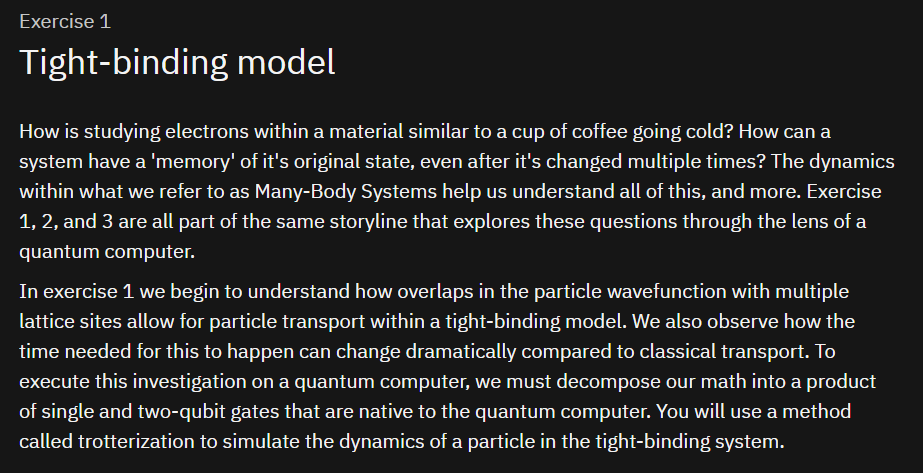
The tight-binding model is a quantum mechanical picture used to describe the conductance of electrons in solid-state materials
We kick off the event by being introduced to the main formula that will be referred to throughout the first three notebooks - our tight-binding Hamiltonian.
$$H_{\rm tb}/\hbar = \sum_i \epsilon_i Z_i + J \sum_{\langle i,j \rangle} (X_i X_j + Y_i Y_j)$$
This equation will be used to model electrons moving in a solid-state material. Basically this is the equation that defines the energy required for atoms to exist at a given site, and the energy required for it to move from one site to another.

Throughout the exercises we will simplify this by taking the assumption of a uniform lattice - where all energies are equal (\(\epsilon_i = 0\)). We will also simplify our example by assuming that the energy required to move from a site to its neighbors, \(J\) is 1. With those assumptions we will explore the time evolution of the Hamiltonian.
We are given the Qiskit implementation of the Hamiltonian and graph out the time evolution of it:
def H_tb():
    # Interactions (I is the identity matrix; X and Y are Pauli matricies; ^ is a tensor product)
    XXs = (I^X^X) + (X^X^I)
    YYs = (I^Y^Y) + (Y^Y^I)

    # Sum interactions
    H = J*(XXs + YYs)

    # Return Hamiltonian
    return H
However before we can execute the unitary time evolution on a quantum computing circuit, we need to decompose this into single and two-gates native to the quantum computer. We can accomplish this using Trotterization. The notebook steps us through the decomposition, to ultimately get the Trotterized version:
$$ U_{\text{tb}}(t) \approx \left[XX\left(\frac{2t}{n}\right)^{(0,1)} YY\left(\frac{2t}{n}\right)^{(0,1)} XX\left(\frac{2t}{n}\right)^{(1,2)} YY\left(\frac{2t}{n}\right)^{(1,2)}\right]^{n} $$
Building Operators
Our actual challenge is now to work with single and two-qubit gates natively and build the ZZ(t), XX(t), and YY(t) operations. We are given the ZZ(t) operator to act as the base of building the other two.
ZZ_qc.cnot(0,1)
ZZ_qc.rz(2 * t, 1)
ZZ_qc.cnot(0,1) 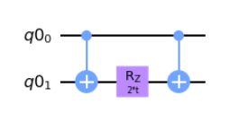
The notebook then reminds us how Clifford gates are used to map Pauli operators to others. This will end up being how we build the remaining operators.
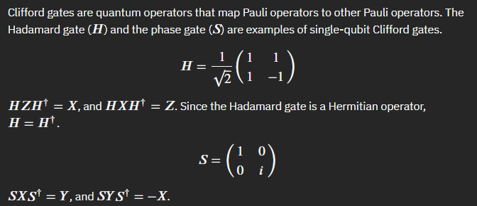
And sure enough, with this information we are then able to build out the XX(t) and YY(t) variants.
###EDIT CODE BELOW (add Clifford operator)
XX_qc.h(0)
XX_qc.h(1)
###DO NOT EDIT BELOW

XX_qc.append(ZZ, [0,1])

###EDIT CODE BELOW (add Clifford operator)
XX_qc.h(0)
XX_qc.h(1)
###DO NOT EDIT BELOW 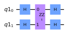
###EDIT CODE BELOW (add Clifford operator)
YY_qc.s(0)
YY_qc.s(1)
YY_qc.h(0)
YY_qc.h(1)
###DO NOT EDIT BELOW

YY_qc.append(ZZ, [0,1])

###EDIT CODE BELOW (add Clifford operator)
YY_qc.h(0)
YY_qc.h(1)
YY_qc.sdg(0)
YY_qc.sdg(1)
###DO NOT EDIT BELOW 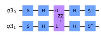
Trotterized Circuit
Great, with our operators built out, the final step in this first notebook is to build the Trotterized evolution circuit. We are given yet one more decomposition which is what we will end up modelling.
$$U(\Delta t) \approx \Big(\prod_{i \in \rm{odd}} e^{-i \Delta t X_iX_{i+1}} e^{-i \Delta t Y_iY_{i+1}} \Big) \Big(\prod_{i \in \rm{even}} e^{-i \Delta t X_iX_{i+1}} e^{-i \Delta t Y_iY_{i+1}} \Big)$$
With the equivalent code.
for i in range(0, num_qubits - 1):
    Trot_qc.append(XX, [Trot_qr[i], Trot_qr[i+1]])
Trot_qc.append(YY, [Trot_qr[i], Trot_qr[i+1]]) 
With this base established we need to complete the function that will build the Trotterized circuit for an arbitrary amount of steps.
def U_trotterize(t_target, trotter_steps):
qr = QuantumRegister(3)
qc = QuantumCircuit(qr)
###EDIT CODE BELOW (Create the trotterized circuit with various number of trotter steps)
for i in range(trotter_steps):
qc.append(Trot_gate, qr)
###DO NOT EDIT BELOW
qc = qc.bind_parameters({t: t_target/trotter_steps})
return qi.Operator(qc)
t_target = 0.5
U_target = U_tb(t_target)
steps=np.arange(1,101,2) ## DO NOT EDIT
fidelities=[]
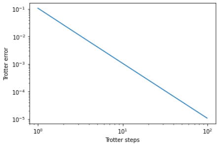
for n in tqdm(steps):
U_trotter = U_trotterize(t_target, trotter_steps=n)
fidelity = qi.process_fidelity(U_trotter, target=U_target)
fidelities.append(fidelity)And sure enough when we graph out the fidelities we see the expect decrease in Trotter errors as we progress through the steps.
Random Walks & Localization
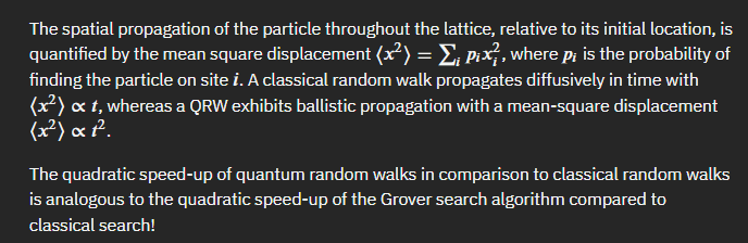
In a tight-binding system the particle propagation can be described by a continuous-time quantum random walk. A random walk is the process by which a randomly-moving particle moves away from its starting point.
One of the reasons we are interested in Quantum Random Walks as opposed to the classical version is the demonstrated speed up experienced. As shown below from the notebook the speed up experienced by this approach demonstrates the same quadratic speed up Grover’s search algorithm presents compared to its classical alternative.
Trotterized Replication
The first step in exploring the Quantum Random Walk is to replicate our Trotterized time evolution circuit from the first notebook, this time on five qubits instead of three. You may be initially confused since the previous equation starts specifies odds and evens. There was some discussion back and forth in the Qiskit slack during the event, however I went with the assumption that the “zeroth” item started as odd, essentially flipping the verbiage.
num_qubits = 5 ## DO NOT EDIT

Trot_tb_qr = QuantumRegister(num_qubits)
Trot_tb_qc = QuantumCircuit(Trot_tb_qr, name='Trot')

###EDIT CODE BELOW
Trot_tb_qc.append(XX,[0,1])
Trot_tb_qc.append(YY,[0,1])

Trot_tb_qc.append(XX,[2,3])
Trot_tb_qc.append(YY,[2,3])

Trot_tb_qc.append(XX,[1,2])
Trot_tb_qc.append(YY,[1,2])

Trot_tb_qc.append(XX,[3,4])
Trot_tb_qc.append(YY,[3,4])
###DO NOT EDIT BELOW 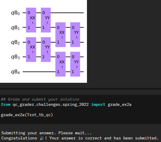
Excitation Probabilities
Great! Now the next step is to excite the first qubit (apply an X gate) and we will then attempt to extract the probabilities of finding the excitation on each qubit at different steps. This is where I started learning more about working with statevectors, specifically being able to pull out probabilities of individual qubits and looking specifically for either the probability of 0 or 1. The capability outputstate.probabilities([qubit])[interested_value] is something I can see myself using in the future even outside of many-body problems.
probability_density=[]
for circ in tqdm(circuits):

    transpiled_circ=transpile(circ, backend_sim, optimization_level=3)

    job_sim = backend_sim.run(transpiled_circ)

    # Grab the results from the job.
    result_sim = job_sim.result()
    outputstate = result_sim.get_statevector(transpiled_circ, decimals=5)

    ps=[]

    ###EDIT CODE BELOW (Extract the probability of finding the excitation on each qubit)
    for i in range(5):
        ps.append(outputstate.probabilities([i])[1])
    ###DO NOT EDIT BELOW

    probability_density.append(ps)

probability_density=np.array(probability_density) 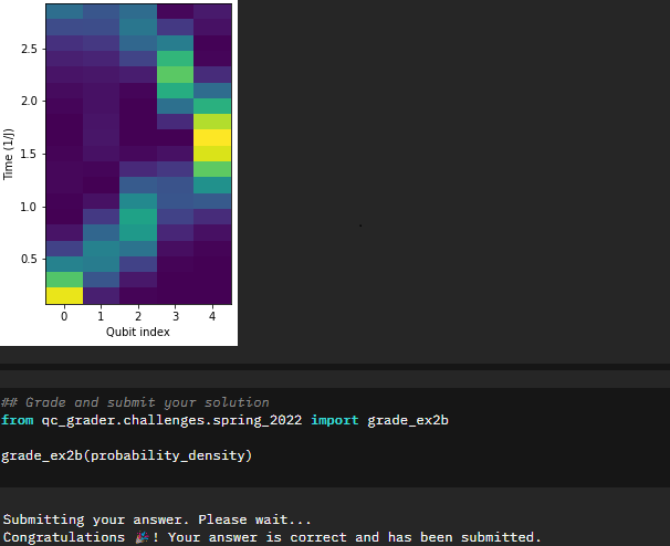
This makes sense if you look back at the initial portions of the notebook. The time evolution of the unitary follows a sinusoidal wave pattern. You can clearly see that pattern if you look at the graph in terms of the time evolution (i.e. flip the graph 90 degrees).
Anderson Localization
The last part of our second notebook will explore Anderson localizations.
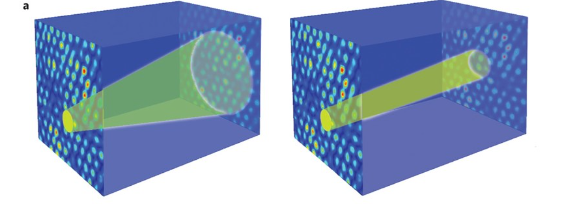
Lattice inhomogeneity causes scattering and leads to quantum interference that tends to inhibit particle propagation, a signature of localization. The wavefunction of a localized particle rapidly decays away from its initial position, effectively confining the particle to a small region of the lattice.
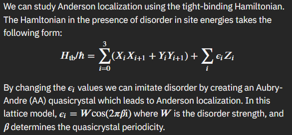
Our challenge is to implement an Anderson Localization to our tight-binding Trotter step circuit. With the equation above we can deduce that we will be applying an Rz rotation with an incorporation of the time evolution. This took a bit of time to figure out how to apply, however if you go back to the first notebook there is a hint in how the original Rz application is done. We can use something similar, adapted for our 5-qubit scenario.
Trot_qc_disorder.append(Trot_tb_gate,[0,1,2,3,4])
deltas=[Parameter('delta_{:d}'.format(idx)) for idx in range(num_qubits)]

###EDIT CODE BELOW (add a parametric disorder to each qubit)
for i in range(num_qubits):
    Trot_qc_disorder.rz(deltas[i]*2*t,i)
###DO NOT EDIT BELOW 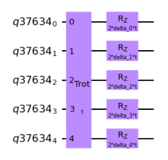
With the Anderson Localization applied, we now want to extract the probabilities of finding an excited state. Based on the localization I would expect it not to be as sinusoidal as before. Let’s take a look.
probability_density_localization=[]
for circ in tqdm(disorder_circuits):

    transpiled_circ=transpile(circ, backend_sim, optimization_level=3)

    job_sim = backend_sim.run(transpiled_circ)

    # Grab the results from the job.
    result_sim = job_sim.result()
    outputstate = result_sim.get_statevector(transpiled_circ, decimals=5)

    ps=[]

    ###EDIT CODE BELOW (Extract the probability of finding the excitation on each qubit)
    for i in range(5):
        ps.append(outputstate.probabilities([i])[1])
    ###DO NOT EDIT BELOW

    probability_density_localization.append(ps)

probability_density_localization=np.array(probability_density_localization) 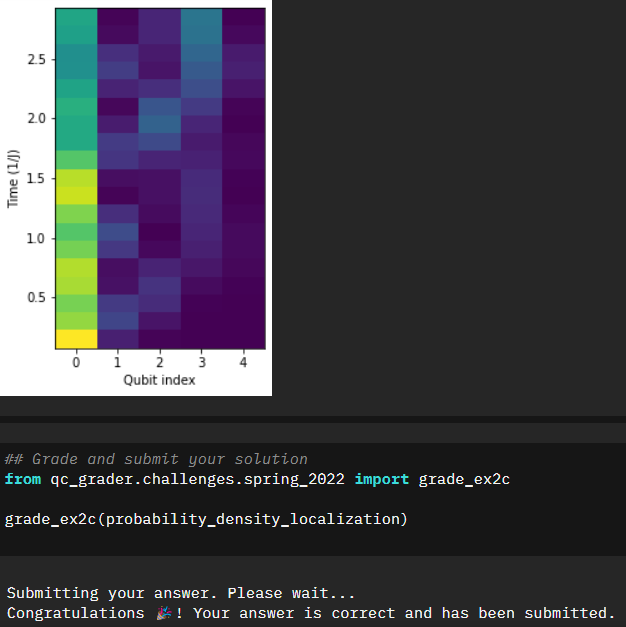
Sure enough that seems to be the result, and our second notebook is successfully completed.
Many-Body Quantum Dynamics
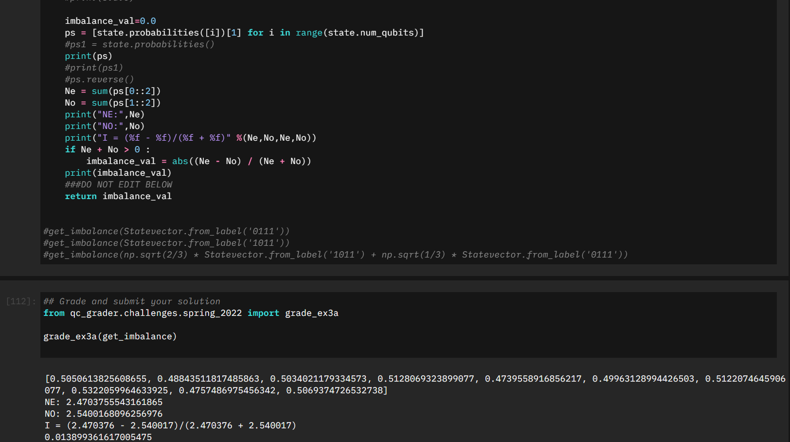
In this exercise we examine lattice disorder and particle-particle interaction. A closed quantum many-body system initialized in a non-equilibrium will reach the equilibrium state, refered to as thermalization, under its own dynamics. This behavior is as a result of the laws of statistical mechanics, and analogous to a hot cup of coffee cooling down to the surrounding temperature if left unattended.
However, the presence of lattice disorder prevents the system from evolving into an egodic thermalized state.
You may be able to see where this is headed. We were able to model the disorder when we explored the Anderson Localizations. By adding multiple excited qubits to the system, we can look for the emergence of imbalance.

Our challenge is to write the function that will calculate the imbalance of an arbitrary quantum state. Arguably this was the most complicated part of the entire event. There was some general confusion at the start with what is considered even/odd, and even when passing the provided test cases successfully, submissions were still not being accepted. While there were discussions from the mentor team on grader oddities (signage errors where -0.0 was not being interpreted the same as 0.0), my particular situation was a logical error. After a bit of discussion with the mentor team I started understanding what I was missing, and I’ll try and capture that in the sections below.
Initial Incorrect Solution
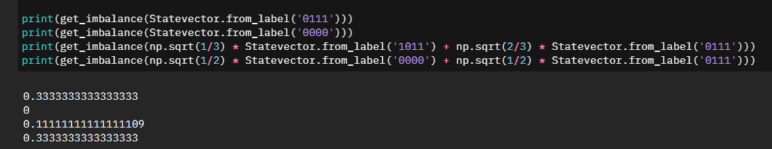
My initial approach was to take the statevector we were given, and similarly pull the probabilities as we did earlier in the challenge:
def get_imbalance(state):
    ###EDIT CODE BELOW
    ### HINT: MAKE SURE TO SKIP CALCULATING IMBALANCE OF THE |00...0> STATE
    imbalance_val=0.0
    ps = [state.probabilities([i])[1] for i in range(state.num_qubits)]

    Ne = sum(ps[0::2])
    No = sum(ps[1::2])

    if Ne + No > 0 :
        imbalance_val = (Ne - No) / (Ne + No)
    ###DO NOT EDIT BELOW

    return imbalance_val
With a bit of tweaking I was testing some of the submissions by taking a look at the statevector, the intermediate values of Ne/No, and ultimately the value of the Imbalance. Despite it looking correct it was still not submitting properly.
It wasn't until I started confirming two very specific test cases that it started making sense. Specifically \(\left|0111\right>\) and \(\left|0000\right> + \left|0111\right>\)
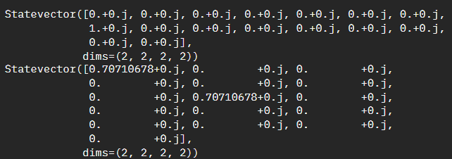
If you are still not following along, essentially with the current code snippet we are summing the probabilities together, however we are not weighing them accordingly. For the above examples our second statevector has a half-weight of \(\left|0000\right>\) which means the imbalance should be half the imbalance value of \(\left|0111\right>\) and half the imbalance value of \(\left|0000\right>\) - which we can see \(\left|0000\right>\) is zero.
We need to repeat the summation as we had done, but we then need to also weigh it by the statevector index itself.Adjusted Solution
With the understanding of what we need to target, I spent a little bit of time creating terrible code to make it work. "Working with numbers is hard? Convert them to Strings!".def get_imbalance(state):
###EDIT CODE BELOW
### HINT: MAKE SURE TO SKIP CALCULATING IMBALANCE OF THE |00...0> STATE
imbalance_val=0
for i in range(2**state.num_qubits):
if state[i] != 0 and i != 0:
num_bits = state.num_qubits
temp = f'{i:0{num_bits}b}'[::-1]
No = 0
Ne = 0
for j in range(num_bits):
if (j % 2) == 0 and temp[j]=="1":
No += 1
elif (j % 2) == 1 and temp[j]=="1":
Ne += 1
imbalance_val += abs(state[i]**2)*((Ne - No) / (Ne + No))
###DO NOT EDIT BELOW
return float(imbalance_val) 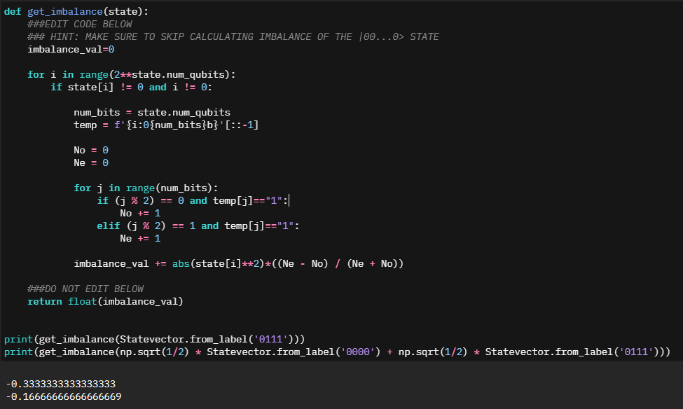
Entropy & Imbalance
With an ability to calculate the imbalance of our system we are then presented with how to calculate the von Neumann entropy - essentially the degree of entanglement of a subsystem and the rest of the system. 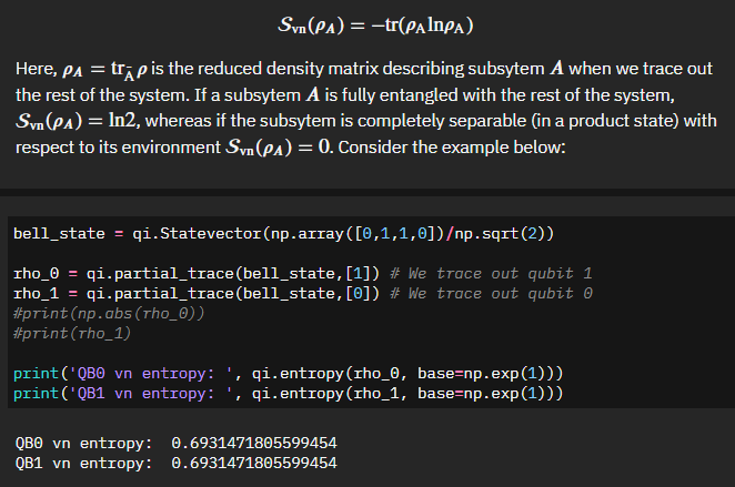
The output here makes sense. Given a bell state, which should be maximally entangled, we get a measurement of 0.69... or \(ln(2)\), which matches our definition. So far so good.
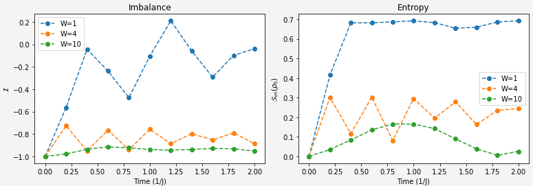
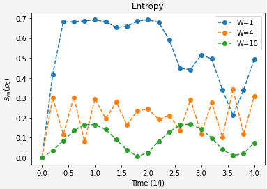
Our two challenges for this section are quite clear:Extract the von Neumann entropy of qubit 0 at different evolution time steps for different disorder strengths.
Extract the imbalance of the lattice at different evolution time steps for different disorder strengths.With our imbalance function and now the clarification on entropy calculation hopefully this is a matter of applying what we already solved to the overall system.
from qiskit import transpile

# Use Aer's statevector simulator
from qiskit import Aer

# Run the quantum circuit on a statevector simulator backend
backend_sim = Aer.get_backend('statevector_simulator')

probability_densities={}
state_vector_imbalances={}
vn_entropies={}

for W in tqdm(Ws):
    probability_densities[W]=[]
    state_vector_imbalances[W]=[]
    vn_entropies[W]=[]

    for circ in circuits[W]:

        transpiled_circ=transpile(circ, backend_sim, optimization_level=3)
        job_sim = backend_sim.run(transpiled_circ)

        # Grab the results from the job.
        result_sim = job_sim.result()
        outputstate = result_sim.get_statevector(transpiled_circ, decimals=6)
        ps=[]
        for idx in range(num_qubits):
            ps.append(np.abs(qi.partial_trace(outputstate,[i for i in range(num_qubits) if i!=idx]))[1,1]**2)

        entropy=0
        ### EDIT CODE BELOW (extract the density matrix of qubit 0 by tracing out all other qubits)
        rho = qi.partial_trace(outputstate,range(1,num_qubits))
        entropy = qi.entropy(rho,base=np.exp(1))
        #print(entropy)
        ###DO NOT EDIT BELOW

        imbalance=0
        ### EDIT CODE BELOW
        imbalance = get_imbalance(outputstate)
        #print(imbalance)
        ###DO NOT EDIT BELOW

        vn_entropies[W].append(entropy)
        probability_densities[W].append(ps)
state_vector_imbalances[W].append(imbalance) 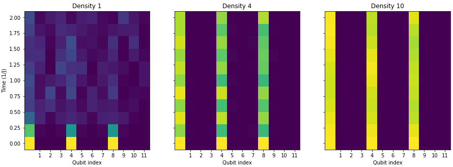
Summary
The Qiskit event was as usual an enlightening event. Having participated in these since early 2020 I can say that these events are a great opportunity to learn hands-on. For myself, I don't have a physics or chemistry background. Much of the challenges to me during this event was trying to simply the exercises down to a simple statement of "what are we trying to implement". With that said, I also wanted to spend time understanding why we were doing this. While I won't say I understand all components, I definitely have a better appreciation than before starting this event. With the release of the fourth notebook shortly after the start of the event, I was able to finish that up as well and finish the Spring 2022 event as part of the first few.